人工智能实践：Tensorflow笔记——深入TensorFlow

本文已收录于 人工智能实践：Tensorflow笔记 系列，共计 7 篇，本篇是第 2 篇

本文已收录到：人工智能实践：Tensorflow笔记 专题

• 人工智能实践：Tensorflow笔记——开篇语
• 人工智能实践：Tensorflow笔记——初识TensorFlow
• 人工智能实践：Tensorflow笔记——深入TensorFlow
• 人工智能实践：Tensorflow笔记——使用八股搭建神经网络
• 人工智能实践：Tensorflow笔记——神经网络八股拓展
• 人工智能实践：Tensorflow笔记——卷积神经网络
• 人工智能实践：Tensorflow笔记——循环神经网络

文章目录 隐藏

1 预备知识

1.1 tf.where()

1.2 np.random.RandomState.rand()

1.3 np.vstack()

1.4 生成网格坐标点

2 复杂度和学习率

2.1 神经网络复杂度

2.2 学习率

3 激活函数

3.1 什么样的激活函数才优秀？

3.2 Sigmoid函数

3.3 Tanh函数

3.4 Relu函数

3.5 Leaky Relu函数

3.6 总结

4 损失函数

4.1 均方误差MES

4.2 自定义损失函数

4.3 交叉熵损失函数

4.4 交叉熵损失函数与softmax结合

5 过拟合与欠拟合

5.1 正则化：缓解过拟合

6 神经网络参数优化器：引导神经网络更新参数的工具

6.1 SGD 随机梯度下降

6.2 SGDM

6.3 Adagrad

6.4 RMSProp

6.5 Adam

6.6 优化器对比

6.6.1 SGD

6.6.2 SGDM

6.6.3 Adagrad

6.6.4 RMSProp

6.6.5 Adam

预备知识

tf.where()

条件语句真返回A,条件语句假返回B

tf.where(条件语句，真返回A，假返回B)

代码示例

import tensorflow as tf

a = tf.constant([1, 2, 3, 1, 1])
b = tf.constant([0, 1, 3, 4, 5])
c = tf.where(tf.greater(a, b), a, b)  # greater函数判断a > b，若a > b，返回a对应位置的元素，否则返回b对应位置的元素
print("c：", c)

1. import tensorflow as tf
3. a = tf.constant([1, 2, 3, 1, 1])
4. b = tf.constant([0, 1, 3, 4, 5])
5. c = tf.where(tf.greater(a, b), a, b) # greater函数判断a > b，若a > b，返回a对应位置的元素，否则返回b对应位置的元素
6. print("c：", c)

import tensorflow as tf

a = tf.constant([1, 2, 3, 1, 1])
b = tf.constant([0, 1, 3, 4, 5])
c = tf.where(tf.greater(a, b), a, b)  # greater函数判断a > b，若a > b，返回a对应位置的元素，否则返回b对应位置的元素
print("c：", c)

运行结果

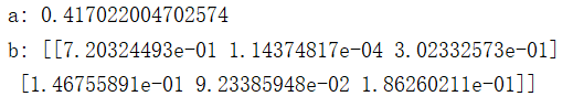
np.random.RandomState.rand()

返回一个[0,1)之间的随机数

np.random.RandomState.rand(维度)  # 若维度为空，返回标量

代码示例

import numpy as np

rdm = np.random.RandomState(seed=1)
a = rdm.rand()
b = rdm.rand(2, 3)
print("a:", a)
print("b:", b)

1. import numpy as np
3. rdm = np.random.RandomState(seed=1)
4. a = rdm.rand()
5. b = rdm.rand(2, 3)
6. print("a:", a)
7. print("b:", b)

import numpy as np

rdm = np.random.RandomState(seed=1)
a = rdm.rand()
b = rdm.rand(2, 3)
print("a:", a)
print("b:", b)

运行结果

np.vstack()

将两个数组按垂直方向叠加

np.vstack(数组1,数组2)

代码示例：

import numpy as np

a = np.array([1, 2, 3])
b = np.array([4, 5, 6])
c = np.vstack((a, b))
print("c:\n", c)

1. import numpy as np
3. a = np.array([1, 2, 3])
4. b = np.array([4, 5, 6])
5. c = np.vstack((a, b))
6. print("c:\n", c)

import numpy as np

a = np.array([1, 2, 3])
b = np.array([4, 5, 6])
c = np.vstack((a, b))
print("c:\n", c)

运行结果

生成网格坐标点

• np.mgrid[ ]
  • np.mgrid[起始值:结束值:步长，起始值:结束值:步长，... ]
  • [起始值，结束值)，区间左闭右开
• x.ravel()将x变为一维数组，“把.前变量拉直”
• np.c_[] 使返回的间隔数值点配对
  • np.c_ [数组1，数组2，... ]

代码示例：

import numpy as np
import tensorflow as tf

# 生成等间隔数值点
x, y = np.mgrid[1:3:1, 2:4:0.5]
# 将x, y拉直，并合并配对为二维张量，生成二维坐标点
grid = np.c_[x.ravel(), y.ravel()]
print("x:\n", x)
print("y:\n", y)
print("x.ravel():\n", x.ravel())
print("y.ravel():\n", y.ravel())
print('grid:\n', grid)

1. import numpy as np
2. import tensorflow as tf
4. # 生成等间隔数值点
5. x, y = np.mgrid[1:3:1, 2:4:0.5]
6. # 将x, y拉直，并合并配对为二维张量，生成二维坐标点
7. grid = np.c_[x.ravel(), y.ravel()]
8. print("x:\n", x)
9. print("y:\n", y)
10. print("x.ravel():\n", x.ravel())
11. print("y.ravel():\n", y.ravel())
12. print('grid:\n', grid)

import numpy as np
import tensorflow as tf

# 生成等间隔数值点
x, y = np.mgrid[1:3:1, 2:4:0.5]
# 将x, y拉直，并合并配对为二维张量，生成二维坐标点
grid = np.c_[x.ravel(), y.ravel()]
print("x:\n", x)
print("y:\n", y)
print("x.ravel():\n", x.ravel())
print("y.ravel():\n", y.ravel())
print('grid:\n', grid)

运行结果

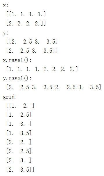
np.mgrid[起始值:结束值:步长，起始值:结束值:步长]填入两个值，相当于构建了一个二维坐标，很坐标值为第一个参数，纵坐标值为第二个参数。

例如，横坐标值为[1, 2, 3]，纵坐标为[2, 2.5, 3, 3.5]

x, y = np.mgrid[1:5:1, 2:4:0.5]
print("x:\n", x)
print("y:\n", y)

这样x和y都为3行4列的二维数组，每个点一一对应构成一个二维坐标区域

x:
 [[1. 1. 1. 1.]
 [2. 2. 2. 2.]
 [3. 3. 3. 3.]]
y:
 [[2.  2.5 3.  3.5]
 [2.  2.5 3.  3.5]
 [2.  2.5 3.  3.5]]

复杂度和学习率

神经网络复杂度

神经网络的复杂度分为空间复杂度和时间复杂度。

 

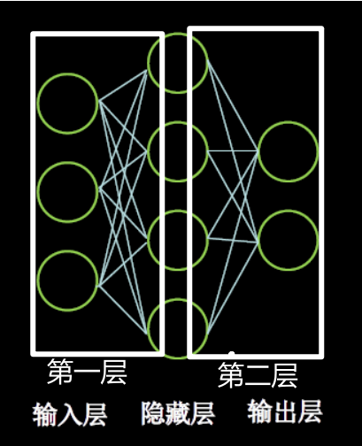
NN复杂度：多用NN层数和NN参数的个数表示

空间复杂度:

层数=隐藏层的层数+ 1个输出层（输入层不参与运算，所以不计算空间复杂度）

图中为：2层NN

总参数=总w+总b

第1层：3×4+4

第2层：4×2+2

图中共计：(3×4+4) +(4×2+2) = 26

时间复杂度:

乘加运算次数

第1层：3×4

第2层：4×2

图中共计：3×4 + 4×2 = 20

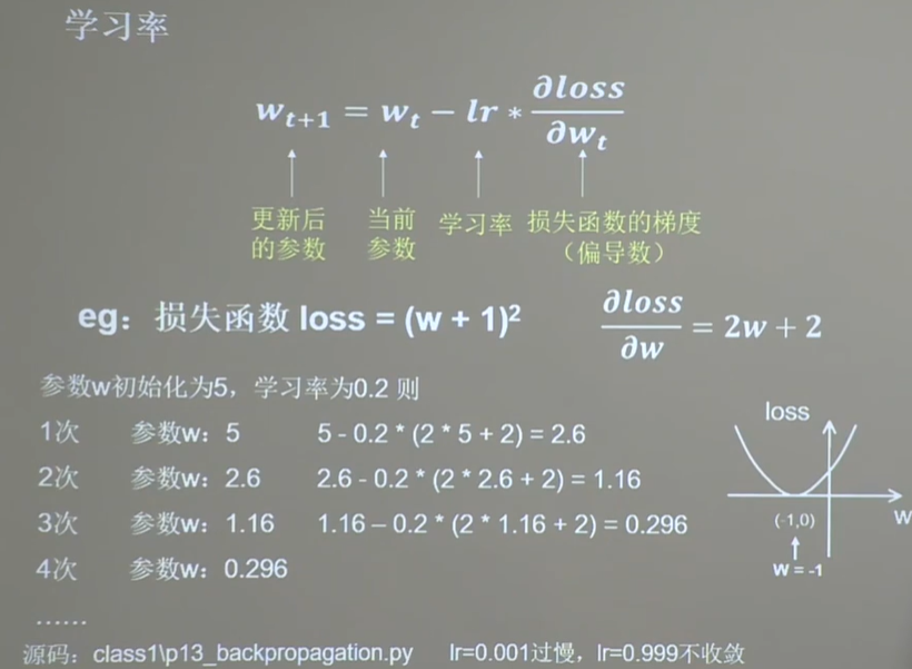
学习率

$$w_{t+1}=w_t-lr\ast \frac{\partial loss}{\partial w_t}$$

参数说明

• 更新后的参数
• 当前参数
• 学习率
• 损失函数的梯度（偏导数）

指数衰减学习率

在之前的学习率部分中，我们发现学习率设置的要么是不收敛、要么是过慢。

在实际使用中如何快速的找到最优解呢？——使用指数衰减学习率。

可以先用较大的学习率，快速得到较优解，然后逐步减小学习率，使模型在训练后期稳定。

上图中绿色部分是超参数。

代码示例

下图白框部分是在原有代码基础上添加的，可以使得学习率指数递减。

运行结果，学习率lr在指数衰减

激活函数

为什么要用激活函数：在神经网络中，如果不对上一层结点的输出做非线性转换的话，再深的网络也是线性模型，只能把输入线性组合再输出，不能学习到复杂的映射关系，因此需要使用激活函数这个非线性函数做转换。

为什么要引入非线性函数，请回顾 –> https://gaozhiyuan.net/machine-learning/artificial-neural-network.html#ren_gong_zhi_neng_de_di_yi_ci_han_dong_ri_chang_zhong_de_hen_duo_wen_ti_shi_fei_xian_xing_ke_fen_de

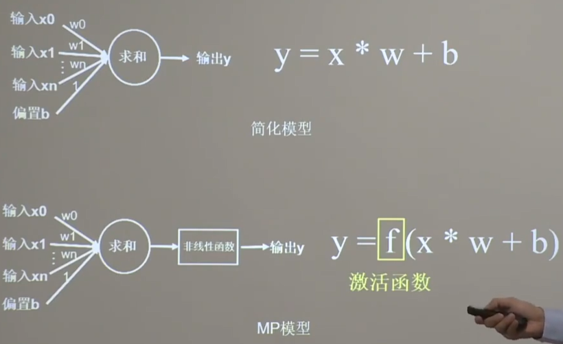
加入了激活函数后可以大大的提高模型的表达能力。

什么样的激活函数才优秀？

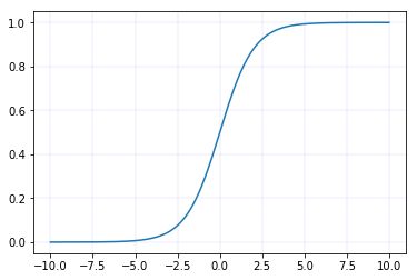
Sigmoid函数

$$\begin{array}{rlr}& \mathrm{sigmod}(x)=\frac{1}{1+e^{-x}}\in (0,1)& {\mathrm{sigmod}}^{\prime }(x)=\mathrm{sigmod}(x{)}^{\ast }(1-\mathrm{sigmod}(x))=\frac{1}{1+e^{-x}}\ast \frac{e^{-x}}{1+e^{-x}}=\frac{e^{-x}}{{(1+e^{-x})}^2}\in (0,0.25)\end{array}$$

tf.nn.sigmoid(x)

sigmoid函数图像

sigmoid导数图像

Ps：目前使用sigmoid函数为激活函数的神经网络已经很少了。

特点

(1)易造成梯度消失

​ 深层神经网络更新参数时，需要从输入层到输出层，逐层进行链式求导，而 sigmoid 函数的导数输出为[0,0.25]间的小数，链式求导需要多层导数连续相乘，这样会出现多个[0,0.25]间的小数连续相乘，从而造成结果趋于0，产生梯度消失，使得参数无法继续更新。

(2)输出非0均值，收敛慢

​ 希望输入每层神经网络的特征是以0为均值的小数值，但 sigmoid 函数激活后的数据都时整数，使得收敛变慢。

(3)幂运算复杂，训练时间长

​ sigmoid 函数存在幂运算，计算复杂度大。

Tanh函数

$$\begin{array}{l}\tanh (x)=\frac{1-e^{-2x}}{1+e^{-2x}}\in (-1,1){\tanh }^{\prime }(x)=1-(\tanh (x){)}^2=\frac{4e^{-2x}}{{(1+e^{-2x})}^2}\in (0,1]\end{array}$$

tf.math.tanh(x)

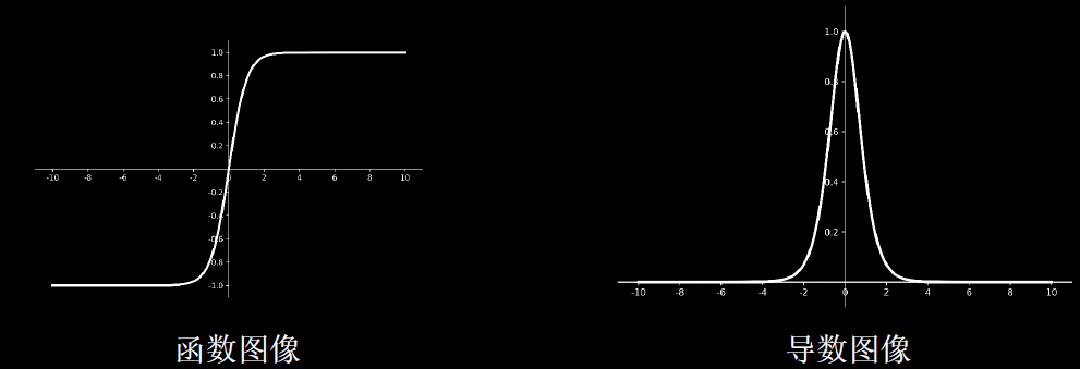
特点

(1)输出是0均值。

(2)依然存在梯度消失问题。

问：什么是梯度？

答：梯度就是矩阵的导数。

问：这里的梯度消失是什么意思？

答：就比如说正方向x有一个很大的数字，例如是100，它对应的y值无限的接近于1。如果是1000，也是无限接近于1。如果我们把这两个x都输出为1的话，就无限体现出他们在x轴上的100和1000接近十倍的差距。——这巨大的差距被忽略了，这就叫梯度消失。从数学的角度来说就是一个很小的数对其求导，求着求着发现无限接近于0了。

(3)幂运算复杂，训练时间长。

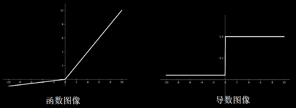
Relu函数

$$\begin{array}{l}relu(x)=max(x,0)=\{\begin{array}{c}x,x\ge 0\\ 0,x<0\end{array}\in [0,+\mathrm{\infty })\\ rel{u}^{\prime }(x)=\{\begin{array}{ll}1,& x\ge 0\\ 0,& x<0\end{array}\in \{0,1\}\end{array}$$

tf.nn.relu(x)

优点:

1. 解决了梯度消失问题（在正区间）
2. 只需判断输入是否大于0，计算速度快。
3. 收敛速度远快于 sigmoid 和 tanh。

缺点:

1. 输出非0均值，收敛慢
2. Dead ReIU问题：某些神经元可能永远不会被激活，导致相应的参数永远不能被更新。所以要避免过多的负数特征进入ReLU函数。

Leaky Relu函数

$$\begin{array}{rl}& \text{ LeakyReLU }(x)=\{\begin{array}{ll}x,& x\ge 0\\ ax,& x<0\end{array}\in R\\ & \text{ LeakyReL }{U}^{\prime }(x)=\{\begin{array}{ll}1,& x\ge 0\\ a,& x<0\end{array}\in \{a,1\}\end{array}$$

tf.nn.leaky_relu(x)

理论上来讲，Leaky Relu有 Relu 的所有优点，外加不会有 Dead Relu 问题，但是在实际操作当中，并没有完全证明 Leaky Relu 总是好于Relu。

总结

• 首选 relu 激活函数;
• 学习率设置较小值;
• 输入特征标准化，即让输入特征满足以0为均值，1为标准差的正态分布;
• 初始参数中心化，即让随机生成的参数满足以0为均值，以$$\sqrt{\frac{2}{\text{ 当前层输入特征个数 }}}$$为标准差的正态分布

损失函数

损失函数(loss) ：预测值(y) 与已知答案(y_) 的差距

NN优化目标：使loss最小。主流的loss有以下三种方法：

• mse (Mean Squared Error)
• 自定义
• ce (Cross Entropy)

均方误差MES

$$\mathrm{MSE}(y_{-},y)=\frac{\sum _{i=1}^n{(y-y_{-})}^2}{n}$$

TensorFlow中使用这个方法来使用MES：loss_mse = tf.reduce_mean(tf.square(y_ - y))

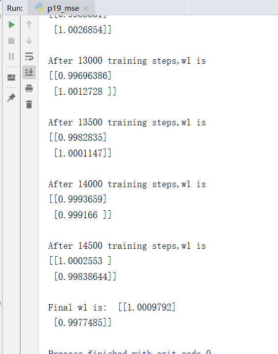
eg：预测酸奶日销量 y，验证 x1和 x2是影响日销量的因素。

建模前，应预先采集的数据有:每日x1、x2和当天的销量y_ （即已知答案，最佳情况:产量=销量）

拟造数据集X，Y_ : y_ =x1 + x2，噪声: -0.05~ +0.05

拟合可以预测销量的函数

代码示例

import tensorflow as tf
import numpy as np

SEED = 23455

rdm = np.random.RandomState(seed=SEED)  # 生成[0,1)之间的随机数
x = rdm.rand(32, 2)                     # 生成32行2列的输入特征x
# 构建标准答案y_
y_ = [[x1 + x2 + (rdm.rand() / 10.0 - 0.05)] for (x1, x2) in x]  # 生成噪声[0,1)/10=[0,0.1); [0,0.1)-0.05=[-0.05,0.05)
x = tf.cast(x, dtype=tf.float32)

w1 = tf.Variable(tf.random.normal([2, 1], stddev=1, seed=1))

epoch = 15000   # 数据集迭代次数
lr = 0.002      # 学习率

for epoch in range(epoch):
    with tf.GradientTape() as tape:
        y = tf.matmul(x, w1)                            # 前向传播结果y
        loss_mse = tf.reduce_mean(tf.square(y_ - y))    # 均方误差

    grads = tape.gradient(loss_mse, w1)                 # 求偏导
    w1.assign_sub(lr * grads)

    if epoch % 500 == 0:
        print("After %d training steps,w1 is " % (epoch))
        print(w1.numpy(), "\n")
print("Final w1 is: ", w1.numpy())

1. import tensorflow as tf
2. import numpy as np
4. SEED = 23455
6. rdm = np.random.RandomState(seed=SEED) # 生成[0,1)之间的随机数
7. x = rdm.rand(32, 2) # 生成32行2列的输入特征x
8. # 构建标准答案y_
9. y_ = [[x1 + x2 + (rdm.rand() / 10.0 - 0.05)] for (x1, x2) in x] # 生成噪声[0,1)/10=[0,0.1); [0,0.1)-0.05=[-0.05,0.05)
10. x = tf.cast(x, dtype=tf.float32)
12. w1 = tf.Variable(tf.random.normal([2, 1], stddev=1, seed=1))
14. epoch = 15000 # 数据集迭代次数
15. lr = 0.002 # 学习率
17. for epoch in range(epoch):
18. with tf.GradientTape() as tape:
19. y = tf.matmul(x, w1) # 前向传播结果y
20. loss_mse = tf.reduce_mean(tf.square(y_ - y)) # 均方误差
22. grads = tape.gradient(loss_mse, w1) # 求偏导
23. w1.assign_sub(lr * grads)
25. if epoch % 500 == 0:
26. print("After %d training steps,w1 is " % (epoch))
27. print(w1.numpy(), "\n")
28. print("Final w1 is: ", w1.numpy())

import tensorflow as tf
import numpy as np

SEED = 23455

rdm = np.random.RandomState(seed=SEED)  # 生成[0,1)之间的随机数
x = rdm.rand(32, 2)                     # 生成32行2列的输入特征x
# 构建标准答案y_
y_ = [[x1 + x2 + (rdm.rand() / 10.0 - 0.05)] for (x1, x2) in x]  # 生成噪声[0,1)/10=[0,0.1); [0,0.1)-0.05=[-0.05,0.05)
x = tf.cast(x, dtype=tf.float32)

w1 = tf.Variable(tf.random.normal([2, 1], stddev=1, seed=1))

epoch = 15000   # 数据集迭代次数
lr = 0.002      # 学习率

for epoch in range(epoch):
    with tf.GradientTape() as tape:
        y = tf.matmul(x, w1)                            # 前向传播结果y
        loss_mse = tf.reduce_mean(tf.square(y_ - y))    # 均方误差

    grads = tape.gradient(loss_mse, w1)                 # 求偏导
    w1.assign_sub(lr * grads)

    if epoch % 500 == 0:
        print("After %d training steps,w1 is " % (epoch))
        print(w1.numpy(), "\n")
print("Final w1 is: ", w1.numpy())

 

运行结果

自定义损失函数

预测商品的销量，预测多了，损失成本。但如果预测少了，损失利润。一般情况下利润≠成本，使用MSE产生的loss无法使得利益最大化。

所以我们尝试使用自定义的损失函数。

自定义损失函数，y_：标准答案数据集的，y：预测答案计算出的 $$\mathrm{loss}\left(y_{-}y\right)=\sum _{n}f\left(y_{，}y\right)$$

把损失定义为一个分段函数：

$$f(y_{-},y)=\{\begin{array}{lll}\text{ PROFIT* }(y_{-}-y)& y<y_{-}& \text{预测的 }y\text{ 少了, 损失利高(PROFIT) }\\ \text{ COST }\ast (y-y_{-})& y>=y_{-}& \text{预测的 }y\text{ 多了，损失成本(COST) }\end{array}$$

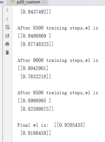
如:预测酸奶销量，酸奶成本(COST) 1元，酸奶利润(PROFIT) 99元。

预测少了损失利润99元，大于预测多了损失成本1元。预测少了损失大，希望生成的预测函数往多了预测。

则损失函数为

loss = tf.reduce_sum(tf.where(tf.greater(y, y_), (y - y_) * COST, (y_ - y) * PROFIT))

代码示例

import tensorflow as tf
import numpy as np

SEED = 23455
COST = 99
PROFIT = 1

rdm = np.random.RandomState(SEED)
x = rdm.rand(32, 2)
y_ = [[x1 + x2 + (rdm.rand() / 10.0 - 0.05)] for (x1, x2) in x]  # 生成噪声[0,1)/10=[0,0.1); [0,0.1)-0.05=[-0.05,0.05)
x = tf.cast(x, dtype=tf.float32)

w1 = tf.Variable(tf.random.normal([2, 1], stddev=1, seed=1))

epoch = 10000
lr = 0.002

for epoch in range(epoch):
    with tf.GradientTape() as tape:
        y = tf.matmul(x, w1)
        loss = tf.reduce_sum(tf.where(tf.greater(y, y_), (y - y_) * COST, (y_ - y) * PROFIT))

    grads = tape.gradient(loss, w1)
    w1.assign_sub(lr * grads)

    if epoch % 500 == 0:
        print("After %d training steps,w1 is " % (epoch))
        print(w1.numpy(), "\n")
print("Final w1 is: ", w1.numpy())

# 自定义损失函数
# 酸奶成本1元， 酸奶利润99元
# 成本很低，利润很高，人们希望多预测些，生成模型系数大于1，往多了预测

1. import tensorflow as tf
2. import numpy as np
4. SEED = 23455
5. COST = 99
6. PROFIT = 1
8. rdm = np.random.RandomState(SEED)
9. x = rdm.rand(32, 2)
10. y_ = [[x1 + x2 + (rdm.rand() / 10.0 - 0.05)] for (x1, x2) in x] # 生成噪声[0,1)/10=[0,0.1); [0,0.1)-0.05=[-0.05,0.05)
11. x = tf.cast(x, dtype=tf.float32)
13. w1 = tf.Variable(tf.random.normal([2, 1], stddev=1, seed=1))
15. epoch = 10000
16. lr = 0.002
18. for epoch in range(epoch):
19. with tf.GradientTape() as tape:
20. y = tf.matmul(x, w1)
21. loss = tf.reduce_sum(tf.where(tf.greater(y, y_), (y - y_) * COST, (y_ - y) * PROFIT))
23. grads = tape.gradient(loss, w1)
24. w1.assign_sub(lr * grads)
26. if epoch % 500 == 0:
27. print("After %d training steps,w1 is " % (epoch))
28. print(w1.numpy(), "\n")
29. print("Final w1 is: ", w1.numpy())
31. # 自定义损失函数
32. # 酸奶成本1元， 酸奶利润99元
33. # 成本很低，利润很高，人们希望多预测些，生成模型系数大于1，往多了预测

import tensorflow as tf
import numpy as np

SEED = 23455
COST = 99
PROFIT = 1

rdm = np.random.RandomState(SEED)
x = rdm.rand(32, 2)
y_ = [[x1 + x2 + (rdm.rand() / 10.0 - 0.05)] for (x1, x2) in x]  # 生成噪声[0,1)/10=[0,0.1); [0,0.1)-0.05=[-0.05,0.05)
x = tf.cast(x, dtype=tf.float32)

w1 = tf.Variable(tf.random.normal([2, 1], stddev=1, seed=1))

epoch = 10000
lr = 0.002

for epoch in range(epoch):
    with tf.GradientTape() as tape:
        y = tf.matmul(x, w1)
        loss = tf.reduce_sum(tf.where(tf.greater(y, y_), (y - y_) * COST, (y_ - y) * PROFIT))

    grads = tape.gradient(loss, w1)
    w1.assign_sub(lr * grads)

    if epoch % 500 == 0:
        print("After %d training steps,w1 is " % (epoch))
        print(w1.numpy(), "\n")
print("Final w1 is: ", w1.numpy())

# 自定义损失函数
# 酸奶成本1元， 酸奶利润99元
# 成本很低，利润很高，人们希望多预测些，生成模型系数大于1，往多了预测

自定义损失函数，酸奶成本1元， 酸奶利润99元，成本很低，利润很高，人们希望多预测些，生成模型系数大于1，往多了预测。运行结果

自定义损失函数，酸奶成本99元， 酸奶利润1元，成本很高，利润很低，人们希望多少预测，生成模型系数小于1，往少了预测。运行结果

交叉熵损失函数

交义熵损失函数CE (Cross Entropy)可以表示两个概率分布之间的距离 $$\mathrm{H}({\mathrm{y}}_{-},\mathrm{y})=-\sum y_{-}\ast \ln y$$

交叉熵越大，两个概率分布越远；交叉熵越小表示两个概率分布越近。

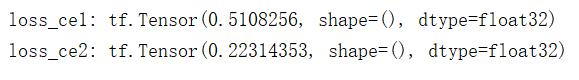
eg：二分类问题，已知答案y_ 有两个取值，一个是1一个是0，预测 y1=(0.6, 0.4)  y2=(0.8, 0.2) ，请问哪个更接近标准答案呢？——直觉上是y2更仅仅标准答案。

$$\begin{array}{rl}& {\mathrm{H}}_1((1,0),(0.6,0.4))=-(1\ast \ln 0.6+0\ast \ln 0.4)\approx -(-0.511+0)=0.511\\ & {\mathrm{H}}_2((1,0),(0.8,0.2))=-(1\ast \ln 0.8+0\ast \ln 0.2)\approx -(-0.223+0)=0.223\end{array}$$

计算得到y1与标准答案的距离是0.511，y2与标准答案的距离是0.223。因为 H2<H1，所以y2预测更准。

tf.losses.categorical crossentropy(y_ ，y)

代码示例

import tensorflow as tf

loss_ce1 = tf.losses.categorical_crossentropy([1, 0], [0.6, 0.4])
loss_ce2 = tf.losses.categorical_crossentropy([1, 0], [0.8, 0.2])
print("loss_ce1:", loss_ce1)
print("loss_ce2:", loss_ce2)

# 交叉熵损失函数

1. import tensorflow as tf
3. loss_ce1 = tf.losses.categorical_crossentropy([1, 0], [0.6, 0.4])
4. loss_ce2 = tf.losses.categorical_crossentropy([1, 0], [0.8, 0.2])
5. print("loss_ce1:", loss_ce1)
6. print("loss_ce2:", loss_ce2)
8. # 交叉熵损失函数

import tensorflow as tf

loss_ce1 = tf.losses.categorical_crossentropy([1, 0], [0.6, 0.4])
loss_ce2 = tf.losses.categorical_crossentropy([1, 0], [0.8, 0.2])
print("loss_ce1:", loss_ce1)
print("loss_ce2:", loss_ce2)

# 交叉熵损失函数

# 交叉熵损失函数

运行结果

交叉熵损失函数与softmax结合

我们在执行分类问题时，通常先用softmax函数使输出结果符合概率分布，再求交叉熵损失函数。

TensorFlow给出了一个可以同时计算概率分布和交叉熵的函数：

tf.nn.softmax_cross_entropy_with_logits(y_, y)

代码示例

# softmax与交叉熵损失函数的结合
import tensorflow as tf
import numpy as np

y_ = np.array([[1, 0, 0], [0, 1, 0], [0, 0, 1], [1, 0, 0], [0, 1, 0]])
y = np.array([[12, 3, 2], [3, 10, 1], [1, 2, 5], [4, 6.5, 1.2], [3, 6, 1]])

y_pro = tf.nn.softmax(y)
loss_ce1 = tf.losses.categorical_crossentropy(y_,y_pro)

# 下面这句可以替代 第8、9行代码
loss_ce2 = tf.nn.softmax_cross_entropy_with_logits(y_, y)   # 一次完成概率分布和交叉熵计算

print('分步计算的结果:\n', loss_ce1)
print('结合计算的结果:\n', loss_ce2)


# 输出的结果相同

1. # softmax与交叉熵损失函数的结合
2. import tensorflow as tf
3. import numpy as np
5. y_ = np.array([[1, 0, 0], [0, 1, 0], [0, 0, 1], [1, 0, 0], [0, 1, 0]])
6. y = np.array([[12, 3, 2], [3, 10, 1], [1, 2, 5], [4, 6.5, 1.2], [3, 6, 1]])
8. y_pro = tf.nn.softmax(y)
9. loss_ce1 = tf.losses.categorical_crossentropy(y_,y_pro)
11. # 下面这句可以替代 第8、9行代码
12. loss_ce2 = tf.nn.softmax_cross_entropy_with_logits(y_, y) # 一次完成概率分布和交叉熵计算
14. print('分步计算的结果:\n', loss_ce1)
15. print('结合计算的结果:\n', loss_ce2)
18. # 输出的结果相同

# softmax与交叉熵损失函数的结合
import tensorflow as tf
import numpy as np

y_ = np.array([[1, 0, 0], [0, 1, 0], [0, 0, 1], [1, 0, 0], [0, 1, 0]])
y = np.array([[12, 3, 2], [3, 10, 1], [1, 2, 5], [4, 6.5, 1.2], [3, 6, 1]])

y_pro = tf.nn.softmax(y)
loss_ce1 = tf.losses.categorical_crossentropy(y_,y_pro)

# 下面这句可以替代 第8、9行代码
loss_ce2 = tf.nn.softmax_cross_entropy_with_logits(y_, y)   # 一次完成概率分布和交叉熵计算

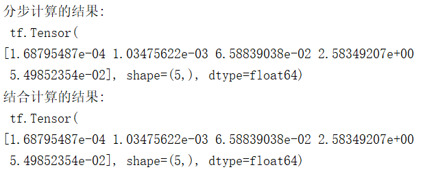
print('分步计算的结果:\n', loss_ce1)
print('结合计算的结果:\n', loss_ce2)


# 输出的结果相同

运行结果

过拟合与欠拟合

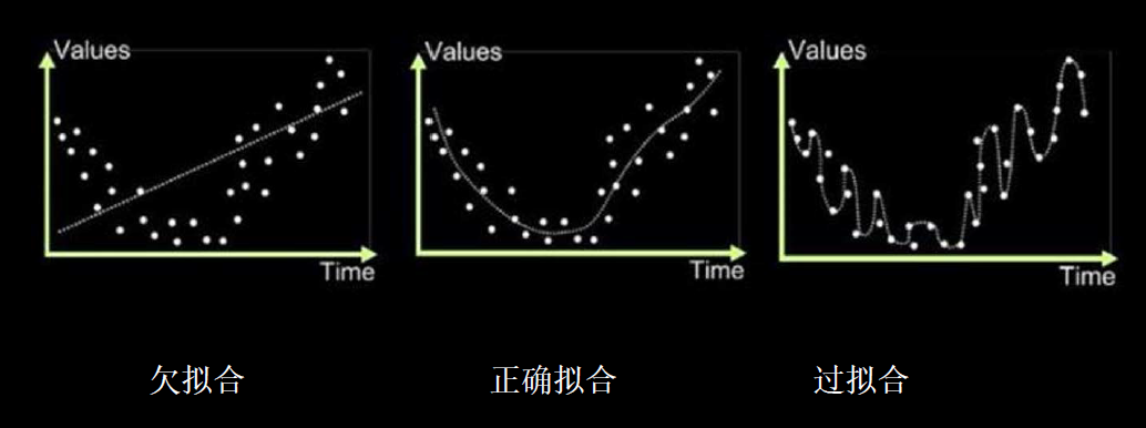
欠拟合：模型不能有效拟合数据集，对现有数据集学习的不彻底。

欠拟合的解决方法:

• 增加输入特征项
• 增加网络参数
• 减少正则化参数

过拟合：模型对当前数据拟合的太好了，见到个新数据却难以做到合适的判断，缺少泛化力。

过拟合的解决方法:

• 数据清洗
• 增大训练集
• 采用正则化
• 增大正则化参数

正则化：缓解过拟合

正则化：在损失函数中引入模型复杂度指标，利用给W加权值，弱化了训练数据的噪声（一般不正则化b）

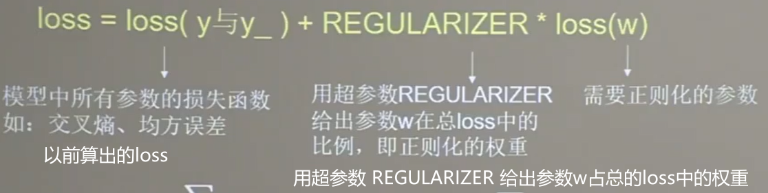
loss(w)是需要正则化的参数。计算方式有两种：

$${\mathrm{loss}}_{L_1}(w)=\sum _i\left|w_i\right|$$

$${\mathrm{loss}}_{L2}(w)=\sum _i\left|w_i^2\right|$$

使用正则化后，loss变成两部分的和。

正则化的选择

• L1正则化大概率会使很多参数变为零，因此该方法可通过稀疏参数，即减少参数的数量，降低复杂度。
• L2正则化会使参数很接近零但不为零，因此该方法可通过减小参数值的大小降低复杂度。

下面来看L2正则化计算loss w的过程：

tf.nn.l2_loss(w)

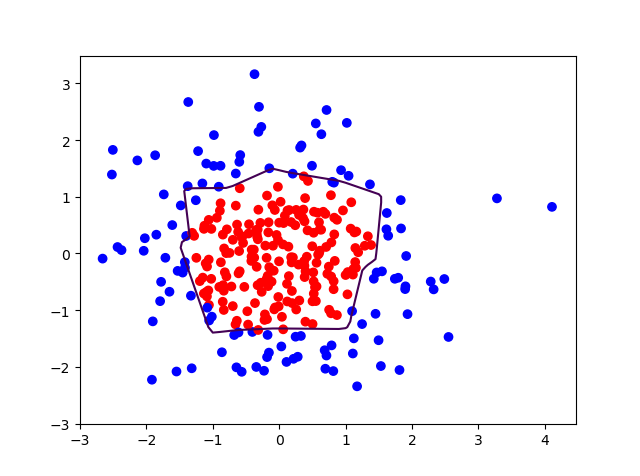
代码示例，未采用正则化p29_regularizationfree.py

# 导入所需模块
import tensorflow as tf
from matplotlib import pyplot as plt
import numpy as np
import pandas as pd

# 读入数据/标签 生成x_train y_train
df = pd.read_csv('dot.csv')
x_data = np.array(df[['x1', 'x2']])
y_data = np.array(df['y_c'])

# reshape(-1,x) -1是将一维数组转换为二维的矩阵，并且第二个参数是表示分成几列，
# 但是在reshape的时候必须让数组里面的个数和shape的函数做取余时值为零才能转换
x_train = np.vstack(x_data).reshape(-1,2)
y_train = np.vstack(y_data).reshape(-1,1)  #将y_data转换为二维数组


Y_c = [['red' if y else 'blue'] for y in y_train]  # 三元运算

# 转换x的数据类型，否则后面矩阵相乘时会因数据类型问题报错
x_train = tf.cast(x_train, tf.float32)
y_train = tf.cast(y_train, tf.float32)

# from_tensor_slices函数切分传入的张量的第一个维度，生成相应的数据集，使输入特征和标签值一一对应
train_db = tf.data.Dataset.from_tensor_slices((x_train, y_train)).batch(32)

# 生成神经网络的参数，输入层为2个神经元，隐藏层为11个神经元，1层隐藏层，输出层为1个神经元
# 隐藏层11个神经元为人为指定
# 用tf.Variable()保证参数可训练
w1 = tf.Variable(tf.random.normal([2, 11]), dtype=tf.float32)  # 隐藏层2个输入，11个输出
b1 = tf.Variable(tf.constant(0.01, shape=[11]))  # b的个数与w个数相同

w2 = tf.Variable(tf.random.normal([11, 1]), dtype=tf.float32)  # 输出层接收11个，输出1个
b2 = tf.Variable(tf.constant(0.01, shape=[1]))

lr = 0.01  # 学习率
epoch = 400  # 循环轮数

# 训练部分
for epoch in range(epoch):
    for step, (x_train, y_train) in enumerate(train_db):
        with tf.GradientTape() as tape:  # 记录梯度信息

            h1 = tf.matmul(x_train, w1) + b1  # 记录神经网络乘加运算
            h1 = tf.nn.relu(h1)  # relu激活函数
            y = tf.matmul(h1, w2) + b2

            # 采用均方误差损失函数mse = mean(sum(y-out)^2)
            loss = tf.reduce_mean(tf.square(y_train - y))

        # 计算loss对各个参数的梯度
        variables = [w1, b1, w2, b2]
        grads = tape.gradient(loss, variables)

        # 实现梯度更新
        # w1 = w1 - lr * w1_grad tape.gradient是自动求导结果与[w1, b1, w2, b2] 索引为0，1，2，3 
        w1.assign_sub(lr * grads[0])
        b1.assign_sub(lr * grads[1])
        w2.assign_sub(lr * grads[2])
        b2.assign_sub(lr * grads[3])

    # 每20个epoch，打印loss信息
    if epoch % 20 == 0:
        print('epoch:', epoch, 'loss:', float(loss))

# 预测部分
print("*******predict*******")
# xx在-3到3之间以步长为0.01，yy在-3到3之间以步长0.01,生成间隔数值点
xx, yy = np.mgrid[-3:3:.1, -3:3:.1]
# 将xx , yy拉直，并合并配对为二维张量，生成二维坐标点
grid = np.c_[xx.ravel(), yy.ravel()]
grid = tf.cast(grid, tf.float32)
# 将网格坐标点喂入神经网络，进行预测，probs为输出
probs = []
for x_test in grid:
    # 使用训练好的参数进行预测
    h1 = tf.matmul([x_test], w1) + b1
    h1 = tf.nn.relu(h1)
    y = tf.matmul(h1, w2) + b2  # y为预测结果
    probs.append(y)

# 取第0列给x1，取第1列给x2
x1 = x_data[:, 0]
x2 = x_data[:, 1]
# probs的shape调整成xx的样子
probs = np.array(probs).reshape(xx.shape)
plt.scatter(x1, x2, color=np.squeeze(Y_c)) # squeeze去掉纬度是1的纬度,相当于去掉[['red'],['blue']],内层括号变为['red','blue']
# 把坐标xx yy和对应的值probs放入contour<[‘kɑntʊr]>函数，给probs值为0.5的所有点上色  plt点show后 显示的是红蓝点的分界线
plt.contour(xx, yy, probs, levels=[.5])  # 画出probs值为0.5轮廓线,levels:这个参数用于显示具体哪几条登高线
plt.show()

# 读入红蓝点，画出分割线，不包含正则化
# 不清楚的数据，建议print出来查看

1. # 导入所需模块
2. import tensorflow as tf
3. from matplotlib import pyplot as plt
4. import numpy as np
5. import pandas as pd
7. # 读入数据/标签 生成x_train y_train
8. df = pd.read_csv('dot.csv')
9. x_data = np.array(df[['x1', 'x2']])
10. y_data = np.array(df['y_c'])
12. # reshape(-1,x) -1是将一维数组转换为二维的矩阵，并且第二个参数是表示分成几列，
13. # 但是在reshape的时候必须让数组里面的个数和shape的函数做取余时值为零才能转换
14. x_train = np.vstack(x_data).reshape(-1,2)
15. y_train = np.vstack(y_data).reshape(-1,1) #将y_data转换为二维数组
18. Y_c = [['red' if y else 'blue'] for y in y_train] # 三元运算
20. # 转换x的数据类型，否则后面矩阵相乘时会因数据类型问题报错
21. x_train = tf.cast(x_train, tf.float32)
22. y_train = tf.cast(y_train, tf.float32)
24. # from_tensor_slices函数切分传入的张量的第一个维度，生成相应的数据集，使输入特征和标签值一一对应
25. train_db = tf.data.Dataset.from_tensor_slices((x_train, y_train)).batch(32)
27. # 生成神经网络的参数，输入层为2个神经元，隐藏层为11个神经元，1层隐藏层，输出层为1个神经元
28. # 隐藏层11个神经元为人为指定
29. # 用tf.Variable()保证参数可训练
30. w1 = tf.Variable(tf.random.normal([2, 11]), dtype=tf.float32) # 隐藏层2个输入，11个输出
31. b1 = tf.Variable(tf.constant(0.01, shape=[11])) # b的个数与w个数相同
33. w2 = tf.Variable(tf.random.normal([11, 1]), dtype=tf.float32) # 输出层接收11个，输出1个
34. b2 = tf.Variable(tf.constant(0.01, shape=[1]))
36. lr = 0.01 # 学习率
37. epoch = 400 # 循环轮数
39. # 训练部分
40. for epoch in range(epoch):
41. for step, (x_train, y_train) in enumerate(train_db):
42. with tf.GradientTape() as tape: # 记录梯度信息
44. h1 = tf.matmul(x_train, w1) + b1 # 记录神经网络乘加运算
45. h1 = tf.nn.relu(h1) # relu激活函数
46. y = tf.matmul(h1, w2) + b2
48. # 采用均方误差损失函数mse = mean(sum(y-out)^2)
49. loss = tf.reduce_mean(tf.square(y_train - y))
51. # 计算loss对各个参数的梯度
52. variables = [w1, b1, w2, b2]
53. grads = tape.gradient(loss, variables)
55. # 实现梯度更新
56. # w1 = w1 - lr * w1_grad tape.gradient是自动求导结果与[w1, b1, w2, b2] 索引为0，1，2，3
57. w1.assign_sub(lr * grads[0])
58. b1.assign_sub(lr * grads[1])
59. w2.assign_sub(lr * grads[2])
60. b2.assign_sub(lr * grads[3])
62. # 每20个epoch，打印loss信息
63. if epoch % 20 == 0:
64. print('epoch:', epoch, 'loss:', float(loss))
66. # 预测部分
67. print("*******predict*******")
68. # xx在-3到3之间以步长为0.01，yy在-3到3之间以步长0.01,生成间隔数值点
69. xx, yy = np.mgrid[-3:3:.1, -3:3:.1]
70. # 将xx , yy拉直，并合并配对为二维张量，生成二维坐标点
71. grid = np.c_[xx.ravel(), yy.ravel()]
72. grid = tf.cast(grid, tf.float32)
73. # 将网格坐标点喂入神经网络，进行预测，probs为输出
74. probs = []
75. for x_test in grid:
76. # 使用训练好的参数进行预测
77. h1 = tf.matmul([x_test], w1) + b1
78. h1 = tf.nn.relu(h1)
79. y = tf.matmul(h1, w2) + b2 # y为预测结果
80. probs.append(y)
82. # 取第0列给x1，取第1列给x2
83. x1 = x_data[:, 0]
84. x2 = x_data[:, 1]
85. # probs的shape调整成xx的样子
86. probs = np.array(probs).reshape(xx.shape)
87. plt.scatter(x1, x2, color=np.squeeze(Y_c)) # squeeze去掉纬度是1的纬度,相当于去掉[['red'],['blue']],内层括号变为['red','blue']
88. # 把坐标xx yy和对应的值probs放入contour<[‘kɑntʊr]>函数，给probs值为0.5的所有点上色 plt点show后 显示的是红蓝点的分界线
89. plt.contour(xx, yy, probs, levels=[.5]) # 画出probs值为0.5轮廓线,levels:这个参数用于显示具体哪几条登高线
90. plt.show()
92. # 读入红蓝点，画出分割线，不包含正则化
93. # 不清楚的数据，建议print出来查看

# 导入所需模块
import tensorflow as tf
from matplotlib import pyplot as plt
import numpy as np
import pandas as pd

# 读入数据/标签 生成x_train y_train
df = pd.read_csv('dot.csv')
x_data = np.array(df[['x1', 'x2']])
y_data = np.array(df['y_c'])

# reshape(-1,x) -1是将一维数组转换为二维的矩阵，并且第二个参数是表示分成几列，
# 但是在reshape的时候必须让数组里面的个数和shape的函数做取余时值为零才能转换
x_train = np.vstack(x_data).reshape(-1,2)
y_train = np.vstack(y_data).reshape(-1,1)  #将y_data转换为二维数组


Y_c = [['red' if y else 'blue'] for y in y_train]  # 三元运算

# 转换x的数据类型，否则后面矩阵相乘时会因数据类型问题报错
x_train = tf.cast(x_train, tf.float32)
y_train = tf.cast(y_train, tf.float32)

# from_tensor_slices函数切分传入的张量的第一个维度，生成相应的数据集，使输入特征和标签值一一对应
train_db = tf.data.Dataset.from_tensor_slices((x_train, y_train)).batch(32)

# 生成神经网络的参数，输入层为2个神经元，隐藏层为11个神经元，1层隐藏层，输出层为1个神经元
# 隐藏层11个神经元为人为指定
# 用tf.Variable()保证参数可训练
w1 = tf.Variable(tf.random.normal([2, 11]), dtype=tf.float32)  # 隐藏层2个输入，11个输出
b1 = tf.Variable(tf.constant(0.01, shape=[11]))  # b的个数与w个数相同

w2 = tf.Variable(tf.random.normal([11, 1]), dtype=tf.float32)  # 输出层接收11个，输出1个
b2 = tf.Variable(tf.constant(0.01, shape=[1]))

lr = 0.01  # 学习率
epoch = 400  # 循环轮数

# 训练部分
for epoch in range(epoch):
    for step, (x_train, y_train) in enumerate(train_db):
        with tf.GradientTape() as tape:  # 记录梯度信息

            h1 = tf.matmul(x_train, w1) + b1  # 记录神经网络乘加运算
            h1 = tf.nn.relu(h1)  # relu激活函数
            y = tf.matmul(h1, w2) + b2

            # 采用均方误差损失函数mse = mean(sum(y-out)^2)
            loss = tf.reduce_mean(tf.square(y_train - y))

        # 计算loss对各个参数的梯度
        variables = [w1, b1, w2, b2]
        grads = tape.gradient(loss, variables)

        # 实现梯度更新
        # w1 = w1 - lr * w1_grad tape.gradient是自动求导结果与[w1, b1, w2, b2] 索引为0，1，2，3 
        w1.assign_sub(lr * grads[0])
        b1.assign_sub(lr * grads[1])
        w2.assign_sub(lr * grads[2])
        b2.assign_sub(lr * grads[3])

    # 每20个epoch，打印loss信息
    if epoch % 20 == 0:
        print('epoch:', epoch, 'loss:', float(loss))

# 预测部分
print("*******predict*******")
# xx在-3到3之间以步长为0.01，yy在-3到3之间以步长0.01,生成间隔数值点
xx, yy = np.mgrid[-3:3:.1, -3:3:.1]
# 将xx , yy拉直，并合并配对为二维张量，生成二维坐标点
grid = np.c_[xx.ravel(), yy.ravel()]
grid = tf.cast(grid, tf.float32)
# 将网格坐标点喂入神经网络，进行预测，probs为输出
probs = []
for x_test in grid:
    # 使用训练好的参数进行预测
    h1 = tf.matmul([x_test], w1) + b1
    h1 = tf.nn.relu(h1)
    y = tf.matmul(h1, w2) + b2  # y为预测结果
    probs.append(y)

# 取第0列给x1，取第1列给x2
x1 = x_data[:, 0]
x2 = x_data[:, 1]
# probs的shape调整成xx的样子
probs = np.array(probs).reshape(xx.shape)
plt.scatter(x1, x2, color=np.squeeze(Y_c)) # squeeze去掉纬度是1的纬度,相当于去掉[['red'],['blue']],内层括号变为['red','blue']
# 把坐标xx yy和对应的值probs放入contour<[‘kɑntʊr]>函数，给probs值为0.5的所有点上色  plt点show后 显示的是红蓝点的分界线
plt.contour(xx, yy, probs, levels=[.5])  # 画出probs值为0.5轮廓线,levels:这个参数用于显示具体哪几条登高线
plt.show()

# 读入红蓝点，画出分割线，不包含正则化
# 不清楚的数据，建议print出来查看

运行结果

epoch: 0 loss: 1.6901788711547852
epoch: 20 loss: 0.06456395983695984
epoch: 40 loss: 0.0639718547463417
epoch: 60 loss: 0.054891664534807205
epoch: 80 loss: 0.037164993584156036
epoch: 100 loss: 0.0290686022490263
epoch: 120 loss: 0.026631897315382957
epoch: 140 loss: 0.025654718279838562
epoch: 160 loss: 0.025450214743614197
epoch: 180 loss: 0.02445397339761257
epoch: 200 loss: 0.02315516769886017
epoch: 220 loss: 0.02262507937848568
epoch: 240 loss: 0.02210732363164425
epoch: 260 loss: 0.02202308177947998
epoch: 280 loss: 0.022013641893863678
epoch: 300 loss: 0.02216213382780552
epoch: 320 loss: 0.02226211130619049
epoch: 340 loss: 0.022413412109017372
epoch: 360 loss: 0.022659024223685265
epoch: 380 loss: 0.02281317301094532
*******predict*******

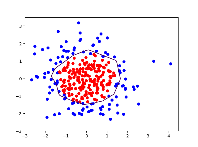
代码示例，在训练部分采用L2正则化

# 导入所需模块
import tensorflow as tf
from matplotlib import pyplot as plt
import numpy as np
import pandas as pd

# 读入数据/标签 生成x_train y_train
df = pd.read_csv('dot.csv')
x_data = np.array(df[['x1', 'x2']])
y_data = np.array(df['y_c'])

x_train = x_data
y_train = y_data.reshape(-1, 1)

Y_c = [['red' if y else 'blue'] for y in y_train]

# 转换x的数据类型，否则后面矩阵相乘时会因数据类型问题报错
x_train = tf.cast(x_train, tf.float32)
y_train = tf.cast(y_train, tf.float32)

# from_tensor_slices函数切分传入的张量的第一个维度，生成相应的数据集，使输入特征和标签值一一对应
train_db = tf.data.Dataset.from_tensor_slices((x_train, y_train)).batch(32)

# 生成神经网络的参数，输入层为4个神经元，隐藏层为32个神经元，2层隐藏层，输出层为3个神经元
# 用tf.Variable()保证参数可训练
w1 = tf.Variable(tf.random.normal([2, 11]), dtype=tf.float32)
b1 = tf.Variable(tf.constant(0.01, shape=[11]))

w2 = tf.Variable(tf.random.normal([11, 1]), dtype=tf.float32)
b2 = tf.Variable(tf.constant(0.01, shape=[1]))

lr = 0.01  # 学习率为
epoch = 400  # 循环轮数

# 训练部分
for epoch in range(epoch):
    for step, (x_train, y_train) in enumerate(train_db):
        with tf.GradientTape() as tape:  # 记录梯度信息

            h1 = tf.matmul(x_train, w1) + b1  # 记录神经网络乘加运算
            h1 = tf.nn.relu(h1)
            y = tf.matmul(h1, w2) + b2

            # 采用均方误差损失函数mse = mean(sum(y-out)^2)
            loss_mse = tf.reduce_mean(tf.square(y_train - y))
            # 添加l2正则化
            loss_regularization = []
            # tf.nn.l2_loss(w)=sum(w ** 2) / 2
            loss_regularization.append(tf.nn.l2_loss(w1))
            loss_regularization.append(tf.nn.l2_loss(w2))
            # 求和
            # 例：x=tf.constant(([1,1,1],[1,1,1]))
            #   tf.reduce_sum(x)
            # >>>6
            # loss_regularization = tf.reduce_sum(tf.stack(loss_regularization))
            loss_regularization = tf.reduce_sum(loss_regularization)
            loss = loss_mse + 0.03 * loss_regularization # REGULARIZER = 0.03

        # 计算loss对各个参数的梯度
        variables = [w1, b1, w2, b2]
        grads = tape.gradient(loss, variables)

        # 实现梯度更新
        # w1 = w1 - lr * w1_grad
        w1.assign_sub(lr * grads[0])
        b1.assign_sub(lr * grads[1])
        w2.assign_sub(lr * grads[2])
        b2.assign_sub(lr * grads[3])

    # 每200个epoch，打印loss信息
    if epoch % 20 == 0:
        print('epoch:', epoch, 'loss:', float(loss))

# 预测部分
print("*******predict*******")
# xx在-3到3之间以步长为0.01，yy在-3到3之间以步长0.01,生成间隔数值点
xx, yy = np.mgrid[-3:3:.1, -3:3:.1]
# 将xx, yy拉直，并合并配对为二维张量，生成二维坐标点
grid = np.c_[xx.ravel(), yy.ravel()]
grid = tf.cast(grid, tf.float32)
# 将网格坐标点喂入神经网络，进行预测，probs为输出
probs = []
for x_predict in grid:
    # 使用训练好的参数进行预测
    h1 = tf.matmul([x_predict], w1) + b1
    h1 = tf.nn.relu(h1)
    y = tf.matmul(h1, w2) + b2  # y为预测结果
    probs.append(y)

# 取第0列给x1，取第1列给x2
x1 = x_data[:, 0]
x2 = x_data[:, 1]
# probs的shape调整成xx的样子
probs = np.array(probs).reshape(xx.shape)
plt.scatter(x1, x2, color=np.squeeze(Y_c))
# 把坐标xx yy和对应的值probs放入contour<[‘kɑntʊr]>函数，给probs值为0.5的所有点上色  plt点show后 显示的是红蓝点的分界线
plt.contour(xx, yy, probs, levels=[.5])
plt.show()

# 读入红蓝点，画出分割线，包含正则化
# 不清楚的数据，建议print出来查看

1. # 导入所需模块
2. import tensorflow as tf
3. from matplotlib import pyplot as plt
4. import numpy as np
5. import pandas as pd
7. # 读入数据/标签 生成x_train y_train
8. df = pd.read_csv('dot.csv')
9. x_data = np.array(df[['x1', 'x2']])
10. y_data = np.array(df['y_c'])
12. x_train = x_data
13. y_train = y_data.reshape(-1, 1)
15. Y_c = [['red' if y else 'blue'] for y in y_train]
17. # 转换x的数据类型，否则后面矩阵相乘时会因数据类型问题报错
18. x_train = tf.cast(x_train, tf.float32)
19. y_train = tf.cast(y_train, tf.float32)
21. # from_tensor_slices函数切分传入的张量的第一个维度，生成相应的数据集，使输入特征和标签值一一对应
22. train_db = tf.data.Dataset.from_tensor_slices((x_train, y_train)).batch(32)
24. # 生成神经网络的参数，输入层为4个神经元，隐藏层为32个神经元，2层隐藏层，输出层为3个神经元
25. # 用tf.Variable()保证参数可训练
26. w1 = tf.Variable(tf.random.normal([2, 11]), dtype=tf.float32)
27. b1 = tf.Variable(tf.constant(0.01, shape=[11]))
29. w2 = tf.Variable(tf.random.normal([11, 1]), dtype=tf.float32)
30. b2 = tf.Variable(tf.constant(0.01, shape=[1]))
32. lr = 0.01 # 学习率为
33. epoch = 400 # 循环轮数
35. # 训练部分
36. for epoch in range(epoch):
37. for step, (x_train, y_train) in enumerate(train_db):
38. with tf.GradientTape() as tape: # 记录梯度信息
40. h1 = tf.matmul(x_train, w1) + b1 # 记录神经网络乘加运算
41. h1 = tf.nn.relu(h1)
42. y = tf.matmul(h1, w2) + b2
44. # 采用均方误差损失函数mse = mean(sum(y-out)^2)
45. loss_mse = tf.reduce_mean(tf.square(y_train - y))
46. # 添加l2正则化
47. loss_regularization = []
48. # tf.nn.l2_loss(w)=sum(w ** 2) / 2
49. loss_regularization.append(tf.nn.l2_loss(w1))
50. loss_regularization.append(tf.nn.l2_loss(w2))
51. # 求和
52. # 例：x=tf.constant(([1,1,1],[1,1,1]))
53. # tf.reduce_sum(x)
54. # >>>6
55. # loss_regularization = tf.reduce_sum(tf.stack(loss_regularization))
56. loss_regularization = tf.reduce_sum(loss_regularization)
57. loss = loss_mse + 0.03 * loss_regularization # REGULARIZER = 0.03
59. # 计算loss对各个参数的梯度
60. variables = [w1, b1, w2, b2]
61. grads = tape.gradient(loss, variables)
63. # 实现梯度更新
64. # w1 = w1 - lr * w1_grad
65. w1.assign_sub(lr * grads[0])
66. b1.assign_sub(lr * grads[1])
67. w2.assign_sub(lr * grads[2])
68. b2.assign_sub(lr * grads[3])
70. # 每200个epoch，打印loss信息
71. if epoch % 20 == 0:
72. print('epoch:', epoch, 'loss:', float(loss))
74. # 预测部分
75. print("*******predict*******")
76. # xx在-3到3之间以步长为0.01，yy在-3到3之间以步长0.01,生成间隔数值点
77. xx, yy = np.mgrid[-3:3:.1, -3:3:.1]
78. # 将xx, yy拉直，并合并配对为二维张量，生成二维坐标点
79. grid = np.c_[xx.ravel(), yy.ravel()]
80. grid = tf.cast(grid, tf.float32)
81. # 将网格坐标点喂入神经网络，进行预测，probs为输出
82. probs = []
83. for x_predict in grid:
84. # 使用训练好的参数进行预测
85. h1 = tf.matmul([x_predict], w1) + b1
86. h1 = tf.nn.relu(h1)
87. y = tf.matmul(h1, w2) + b2 # y为预测结果
88. probs.append(y)
90. # 取第0列给x1，取第1列给x2
91. x1 = x_data[:, 0]
92. x2 = x_data[:, 1]
93. # probs的shape调整成xx的样子
94. probs = np.array(probs).reshape(xx.shape)
95. plt.scatter(x1, x2, color=np.squeeze(Y_c))
96. # 把坐标xx yy和对应的值probs放入contour<[‘kɑntʊr]>函数，给probs值为0.5的所有点上色 plt点show后 显示的是红蓝点的分界线
97. plt.contour(xx, yy, probs, levels=[.5])
98. plt.show()
100. # 读入红蓝点，画出分割线，包含正则化
101. # 不清楚的数据，建议print出来查看

# 导入所需模块
import tensorflow as tf
from matplotlib import pyplot as plt
import numpy as np
import pandas as pd

# 读入数据/标签 生成x_train y_train
df = pd.read_csv('dot.csv')
x_data = np.array(df[['x1', 'x2']])
y_data = np.array(df['y_c'])

x_train = x_data
y_train = y_data.reshape(-1, 1)

Y_c = [['red' if y else 'blue'] for y in y_train]

# 转换x的数据类型，否则后面矩阵相乘时会因数据类型问题报错
x_train = tf.cast(x_train, tf.float32)
y_train = tf.cast(y_train, tf.float32)

# from_tensor_slices函数切分传入的张量的第一个维度，生成相应的数据集，使输入特征和标签值一一对应
train_db = tf.data.Dataset.from_tensor_slices((x_train, y_train)).batch(32)

# 生成神经网络的参数，输入层为4个神经元，隐藏层为32个神经元，2层隐藏层，输出层为3个神经元
# 用tf.Variable()保证参数可训练
w1 = tf.Variable(tf.random.normal([2, 11]), dtype=tf.float32)
b1 = tf.Variable(tf.constant(0.01, shape=[11]))

w2 = tf.Variable(tf.random.normal([11, 1]), dtype=tf.float32)
b2 = tf.Variable(tf.constant(0.01, shape=[1]))

lr = 0.01  # 学习率为
epoch = 400  # 循环轮数

# 训练部分
for epoch in range(epoch):
    for step, (x_train, y_train) in enumerate(train_db):
        with tf.GradientTape() as tape:  # 记录梯度信息

            h1 = tf.matmul(x_train, w1) + b1  # 记录神经网络乘加运算
            h1 = tf.nn.relu(h1)
            y = tf.matmul(h1, w2) + b2

            # 采用均方误差损失函数mse = mean(sum(y-out)^2)
            loss_mse = tf.reduce_mean(tf.square(y_train - y))
            # 添加l2正则化
            loss_regularization = []
            # tf.nn.l2_loss(w)=sum(w ** 2) / 2
            loss_regularization.append(tf.nn.l2_loss(w1))
            loss_regularization.append(tf.nn.l2_loss(w2))
            # 求和
            # 例：x=tf.constant(([1,1,1],[1,1,1]))
            #   tf.reduce_sum(x)
            # >>>6
            # loss_regularization = tf.reduce_sum(tf.stack(loss_regularization))
            loss_regularization = tf.reduce_sum(loss_regularization)
            loss = loss_mse + 0.03 * loss_regularization # REGULARIZER = 0.03

        # 计算loss对各个参数的梯度
        variables = [w1, b1, w2, b2]
        grads = tape.gradient(loss, variables)

        # 实现梯度更新
        # w1 = w1 - lr * w1_grad
        w1.assign_sub(lr * grads[0])
        b1.assign_sub(lr * grads[1])
        w2.assign_sub(lr * grads[2])
        b2.assign_sub(lr * grads[3])

    # 每200个epoch，打印loss信息
    if epoch % 20 == 0:
        print('epoch:', epoch, 'loss:', float(loss))

# 预测部分
print("*******predict*******")
# xx在-3到3之间以步长为0.01，yy在-3到3之间以步长0.01,生成间隔数值点
xx, yy = np.mgrid[-3:3:.1, -3:3:.1]
# 将xx, yy拉直，并合并配对为二维张量，生成二维坐标点
grid = np.c_[xx.ravel(), yy.ravel()]
grid = tf.cast(grid, tf.float32)
# 将网格坐标点喂入神经网络，进行预测，probs为输出
probs = []
for x_predict in grid:
    # 使用训练好的参数进行预测
    h1 = tf.matmul([x_predict], w1) + b1
    h1 = tf.nn.relu(h1)
    y = tf.matmul(h1, w2) + b2  # y为预测结果
    probs.append(y)

# 取第0列给x1，取第1列给x2
x1 = x_data[:, 0]
x2 = x_data[:, 1]
# probs的shape调整成xx的样子
probs = np.array(probs).reshape(xx.shape)
plt.scatter(x1, x2, color=np.squeeze(Y_c))
# 把坐标xx yy和对应的值probs放入contour<[‘kɑntʊr]>函数，给probs值为0.5的所有点上色  plt点show后 显示的是红蓝点的分界线
plt.contour(xx, yy, probs, levels=[.5])
plt.show()

# 读入红蓝点，画出分割线，包含正则化
# 不清楚的数据，建议print出来查看

运行结果

epoch: 0 loss: 1.530280351638794
epoch: 20 loss: 0.7782743573188782
epoch: 40 loss: 0.6781619191169739
epoch: 60 loss: 0.5953636765480042
epoch: 80 loss: 0.5263288617134094
epoch: 100 loss: 0.4674427807331085
epoch: 120 loss: 0.41659849882125854
epoch: 140 loss: 0.37269479036331177
epoch: 160 loss: 0.3337797522544861
epoch: 180 loss: 0.3002385199069977
epoch: 200 loss: 0.27038004994392395
epoch: 220 loss: 0.24350212514400482
epoch: 240 loss: 0.22041508555412292
epoch: 260 loss: 0.20032131671905518
epoch: 280 loss: 0.1829461306333542
epoch: 300 loss: 0.16758175194263458
epoch: 320 loss: 0.15422624349594116
epoch: 340 loss: 0.14259028434753418
epoch: 360 loss: 0.13238896429538727
epoch: 380 loss: 0.12349270284175873
*******predict*******

补充内容：python matplotlib contour画等高线图

https://blog.csdn.net/Mr_Cat123/article/details/80677525

神经网络参数优化器：引导神经网络更新参数的工具

优化器：是引导神经网络更新参数的工具

作用：用来更新和计算影响模型训练和模型输出的网络参数，使其逼近或达到最优值，从而最小化(或最大化)损失函数

待优化参数w，损失函数loss, 学习率lr， 每次迭代个batch（每个batch包含2^n组数据），t表示当前batch迭代的总次数:

1.计算t时刻损失函数关于当前参数的梯度 $$g_t=\mathrm{\nabla }\mathrm{loss}=\frac{\partial \mathrm{loss}}{\partial \left(w_t\right)}$$ 2.计算t时刻一阶动量mt和二阶动量Vt

• 一阶动量:与梯度相关的函数
• 二阶动量:与梯度平方相关的函数

3.计算t时刻下降梯度: $${\eta }_{\mathrm{t}}=lr\cdot m_{\mathrm{t}}/\sqrt{V_{\mathrm{t}}}$$ 4.计算t+1时刻参数 $$w_{\mathrm{t}+1}=w_t-{\eta }_t=w_t-lr\cdot m_t/\sqrt{V_t}$$ 不同的优化器实质上只是定义了不同的一阶动量和二阶动量公式

SGD 随机梯度下降

SGD (无momentum)，常用的梯度下降法。 $$m_{\mathrm{t}}=g_{\mathrm{t}}{V}_{\mathrm{t}}=1$$

$${\mathit{\eta }}_{\mathrm{t}}=\mathit{l}\mathit{r}\cdot {\mathit{m}}_{\mathrm{t}}/\sqrt{{\mathit{V}}_t}=\mathit{l}\mathit{r}\cdot {\mathit{g}}_t$$

$$\begin{array}{rlr}{w}_{t+1}=& w_t-{\eta }_t& =w_t-lr\cdot m_t/\sqrt{v_t}=w_t-lr\cdot g_t\end{array}$$

即为 $$m_{\mathrm{t}}=\beta \cdot m_{t-1}+(1-\beta )\cdot g_t$$

SGDM

( SGDM (含momentum的SGD)，在SGD基础上增加一 阶动量。 $$m_{\mathrm{t}}=\beta \cdot m_{t-1}+(1-\beta )\cdot g_t$$ mt：表示各时刻梯度方向的指数滑动平均值

β：超参数，趋近于1，经验值为0.9 $$V_{\mathrm{t}}=1$$

$$\begin{array}{rlr}{\eta }_{\mathrm{t}}=& \mathrm{lr}\cdot m_{\mathrm{t}}/\sqrt{V_{\mathrm{t}}}=\mathrm{lr}\cdot m_{\mathrm{t}}& =\mathrm{lr}\cdot (\beta \cdot m_{\mathrm{t}-1}+(1-\beta )\cdot g_{\mathrm{t}})\end{array}$$

$$\begin{array}{rlr}{w}_{\mathrm{t}+1}=& w_{\mathrm{t}}-{\eta }_{\mathrm{t}}& =w_{\mathrm{t}}-lr\cdot (\beta \cdot m_{\mathrm{t}-1}+(1-\beta )\cdot g_{\mathrm{t}})\end{array}$$

Adagrad

Adagrad, 在SGD基础上增加二阶动量 $$m_{\mathrm{t}}=g_{\mathrm{t}}$$ 二阶动量是从开始到现在梯度平方的累计和: $$V_t=\sum _{\tau =1}^t{g}_{\tau }^2$$

$$\begin{array}{l}{\eta }_{\mathrm{t}}=lr\cdot m_t/(\sqrt{V_t})=lr\cdot g_t/(\sqrt{\sum _{\tau =1}^t{g}_t^2})\end{array}$$

$$\begin{array}{rlr}{w}_{t+1}=& w_t-{\eta }_t& =w_t-lr\cdot g_t/(\sqrt{\sum _{\tau =1}^t{g}_t^2})\end{array}$$

RMSProp

RMSProp, SGD基础上增加二 阶动量 $$m_{\mathrm{t}}=g_{\mathrm{t}}$$ 二阶动量v使用指数滑动平均值计算，表征的是过去一段时间的平均值 $$V_t=\beta \cdot V_{t-1}+(1-\beta )\cdot g_t^2$$

$$\begin{array}{rlr}{\eta }_t=& lr\cdot m_{\mathrm{t}}/\sqrt{V_{\mathrm{t}}}& =lr\cdot g_t/(\sqrt{\beta \cdot V_{t-1}+(1-\beta )\cdot g_t^2})\end{array}$$

$$\begin{array}{rlr}{w}_{t+1}& =w_t-{\eta }_t& =w_t-lr\cdot g_t/(\sqrt{\beta \cdot V_{t-1}+(1-\beta )\cdot g_t^2})\end{array}$$

Adam

Adam，同时结合SGDM一阶动量和RMSProp二阶动量

一阶动量： $$m_{\mathrm{t}}={\beta }_1\cdot m_{t-1}+(1-{\beta }_1)\cdot g_t$$ 修正一阶动量的偏差，t为从训练开始到当前时刻所经历的总batch数:: $${\hat{m}}_{\mathrm{t}}=\frac{m_{\mathrm{t}}}{1-{\beta }_1^t}$$ 二阶动量： $$V_t={\beta }_2\cdot V_{step-1}+(1-{\beta }_2)\cdot g_t^2$$ 修正二阶动量的偏差，t为从训练开始到当前时刻所经历的总batch数: $$\widehat{V_t}=\frac{V_t}{1-{\beta }_2^t}$$

$$\begin{array}{rl}{\eta }_t=& lr\cdot {\hat{m}}_{\mathrm{t}}/\sqrt{{\hat{V}}_t}\\ & =\mathrm{lr}\cdot \frac{m_{\mathrm{t}}}{1-{\beta }_1^t}/\sqrt{\frac{V_t}{1-{\beta }_2^t}}\end{array}$$

$$\begin{array}{rl}{w}_{t+1}& =w_t-{\eta }_t\\ & =w_t-lr\cdot \frac{m_t}{1-{\beta }_1^t}/\sqrt{\frac{v_t}{1-{\beta }_2^t}}\end{array}$$

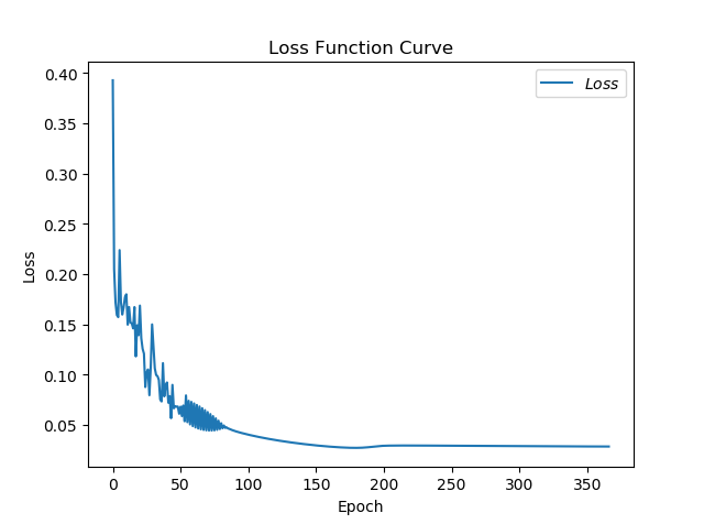
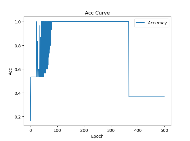
优化器对比

class2中代码p32-p40

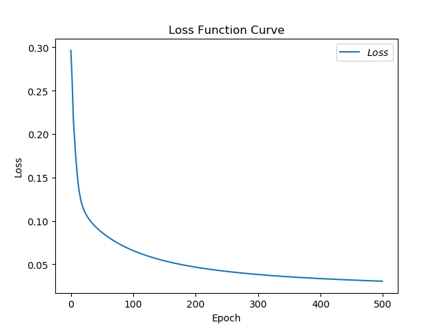
SGD

loss图像

acc图像

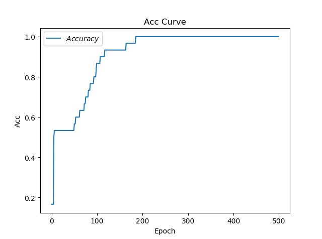
耗时：12.678699254989624

SGDM

loss图像

acc图像

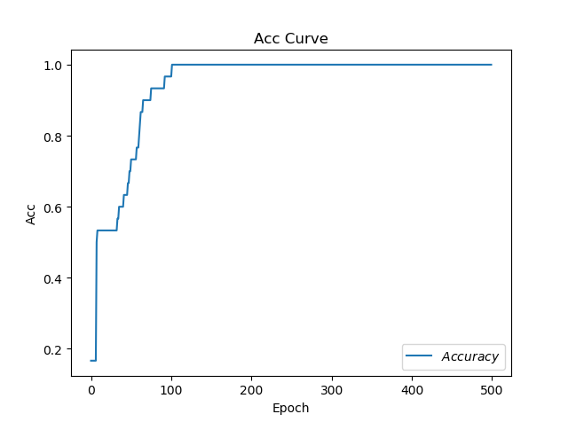
耗时：17.32265305519104

Adagrad

loss图像

acc图像

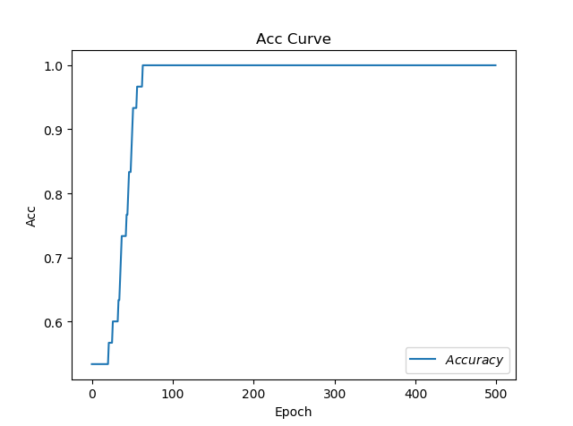
耗时：13.080469131469727

RMSProp

loss图像

acc图像

耗时：16.42955780029297

Adam

loss图像

acc图像

耗时：22.04225492477417

作者： 高志远

高志远，24岁，男生 查看高志远的所有文章