本文已收录到:人工智能实践:Tensorflow笔记 专题
学习目标
①自制数据集,解决自己本领域应用。
②数据量过少,模型训练不足:使用数据增强,扩充数据集。
③断点续训,实时保留当前最优模型。
④神经网络的目的是拿到参数。所以要学会提取参数,把参数存入文本。将来在任何地方可以使用参数构建模型无需训练。
⑤acc/loss可视化,查看训练效果。
⑥应用程序,给图识物。
本章节在此代码中进行拓展:

import tensorflow as tf

mnist = tf.keras.datasets.mnist
(x_train, y_train), (x_test, y_test) = mnist.load_data()
x_train, x_test = x_train / 255.0, x_test / 255.0

model = tf.keras.models.Sequential([
    tf.keras.layers.Flatten(),
    tf.keras.layers.Dense(128, activation='relu'),
    tf.keras.layers.Dense(10, activation='softmax')
])

model.compile(optimizer='adam',
              loss=tf.keras.losses.SparseCategoricalCrossentropy(from_logits=False),
              metrics=['sparse_categorical_accuracy'])

model.fit(x_train, y_train, batch_size=32, epochs=5, validation_data=(x_test, y_test), validation_freq=1)
model.summary()
本讲将在它的基础之上进行改进。
自制数据集
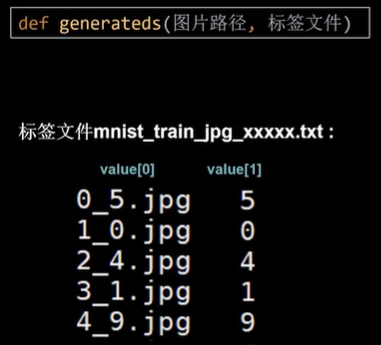
希望通过一个def generateds(图片路径,标签文件)函数获取自定义数据集。
原始图像的文件名是有规律的,下划线右边的数字就是标签,左边的是序列号。所以我们只需要写一个函数将其提取出来就好。
import tensorflow as tf
from PIL import Image
import numpy as np
import os
# 训练集图片路径
train_path = './mnist_image_label/mnist_train_jpg_60000/'
# 训练集标签文件
train_txt = './mnist_image_label/mnist_train_jpg_60000.txt'
# 训练集输入特征存储文件
x_train_savepath = './mnist_image_label/mnist_x_train.npy'
# 训练集标签存储文件
y_train_savepath = './mnist_image_label/mnist_y_train.npy'
# 测试集图片路径
test_path = './mnist_image_label/mnist_test_jpg_10000/'
# 测试集标签文件
test_txt = './mnist_image_label/mnist_test_jpg_10000.txt'
# 测试集输入特征存储文件
x_test_savepath = './mnist_image_label/mnist_x_test.npy'
# 测试集标签存储文件
y_test_savepath = './mnist_image_label/mnist_y_test.npy'
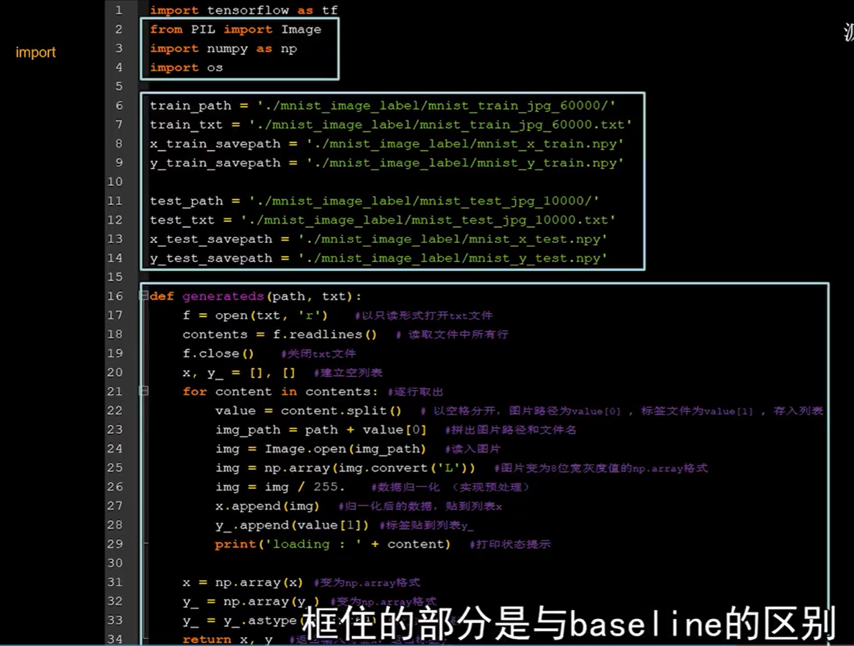
# 处理函数
def generateds(path, txt):
f = open(txt, 'r') # 以只读形式打开txt文件
contents = f.readlines() # 读取文件中所有行
f.close() # 关闭txt文件
x, y_ = [], [] # 建立空列表
for content in contents: # 逐行取出
value = content.split() # 以空格分开,图片路径为value[0] , 标签为value[1] , 存入列表
img_path = path + value[0] # 拼出图片路径和文件名
img = Image.open(img_path) # 读入图片
img = np.array(img.convert('L'))# 图片变为8位宽灰度值的np.array格式
img = img / 255. # 数据归一化 (实现预处理)
x.append(img) # 归一化后的数据,贴到列表x
y_.append(value[1]) # 标签贴到列表y_
print('loading : ' + content) # 打印状态提示
x = np.array(x) # 变为np.array格式
y_ = np.array(y_) # 变为np.array格式
y_ = y_.astype(np.int64) # 变为64位整型
return x, y_ # 返回输入特征x,返回标签y_
if os.path.exists(x_train_savepath) and os.path.exists(y_train_savepath) and os.path.exists(
x_test_savepath) and os.path.exists(y_test_savepath):
print('-------------加载数据集-----------------')
x_train_save = np.load(x_train_savepath)
y_train = np.load(y_train_savepath)
x_test_save = np.load(x_test_savepath)
y_test = np.load(y_test_savepath)
x_train = np.reshape(x_train_save, (len(x_train_save), 28, 28))
x_test = np.reshape(x_test_save, (len(x_test_save), 28, 28))
else:
print('-------------使用 Generate 函数制作数据集-----------------')
x_train, y_train = generateds(train_path, train_txt)
x_test, y_test = generateds(test_path, test_txt)
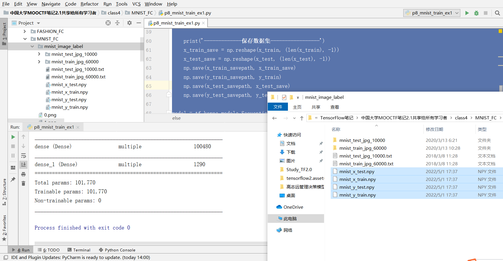
print('-------------保存数据集-----------------')
x_train_save = np.reshape(x_train, (len(x_train), -1))
x_test_save = np.reshape(x_test, (len(x_test), -1))
np.save(x_train_savepath, x_train_save)
np.save(y_train_savepath, y_train)
np.save(x_test_savepath, x_test_save)
np.save(y_test_savepath, y_test)
model = tf.keras.models.Sequential([
tf.keras.layers.Flatten(),
tf.keras.layers.Dense(128, activation='relu'),
tf.keras.layers.Dense(10, activation='softmax')
])
model.compile(optimizer='adam',
loss=tf.keras.losses.SparseCategoricalCrossentropy(from_logits=False),
metrics=['sparse_categorical_accuracy'])
model.fit(x_train, y_train, batch_size=32, epochs=5, validation_data=(x_test, y_test), validation_freq=1)
model.summary()
数据增强
对图像的增强就是对图像进行简单形变,解决因为拍照角度不同等因素造成的影响。
tensorflow2中的数据增强函数
image_gen_train = tf.keras.preprocessing.image.lmageDataGenerator(
	rescale =所有数据将乘以该数值
	rotation_ range =随机旋转角度数范围
	width_ shift range =随机宽度偏移量
	height shift range =随机高度偏移量
	水平翻转: horizontal_flip =是否随机水平翻转
	随机缩放: zoom_range =随机缩放的范围[1-n, 1+n] )

image_gen_train.fit(x_train)
例如
image_gen_train = ImageDataGenerator(
	rescale=1. / 1.,# 如为图像,分母为255时,可归至0 ~ 1
	rotation_ range=45, #随机45度旋转
	width_ shift_ range=.15, #宽度偏移
	height_ shift_ range= .15, #高度偏移
	horizontal_ flip=False, #水平翻转
	zoom range=0.5 # 将图像随机缩放闵量50%)
	image_ gen_train. fit(x_ train)

image_gen_train.fit(x_train)
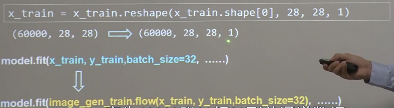
因为上面最后一行 x_train 需要四维数据,所以需要对 x_train 进行 reshape。
把 60000 张 28 行 28 列的数据变为 60000 张 28 行 28 列的单通道数据,最后的1代表灰度值。
model.fit也要做出相应调整。
model.fit(x_train, y_train,batch size=32,...) 变为 model.fit(image_gen_train.flow(x_train, y_train,batch_size=32),...)
代码示例
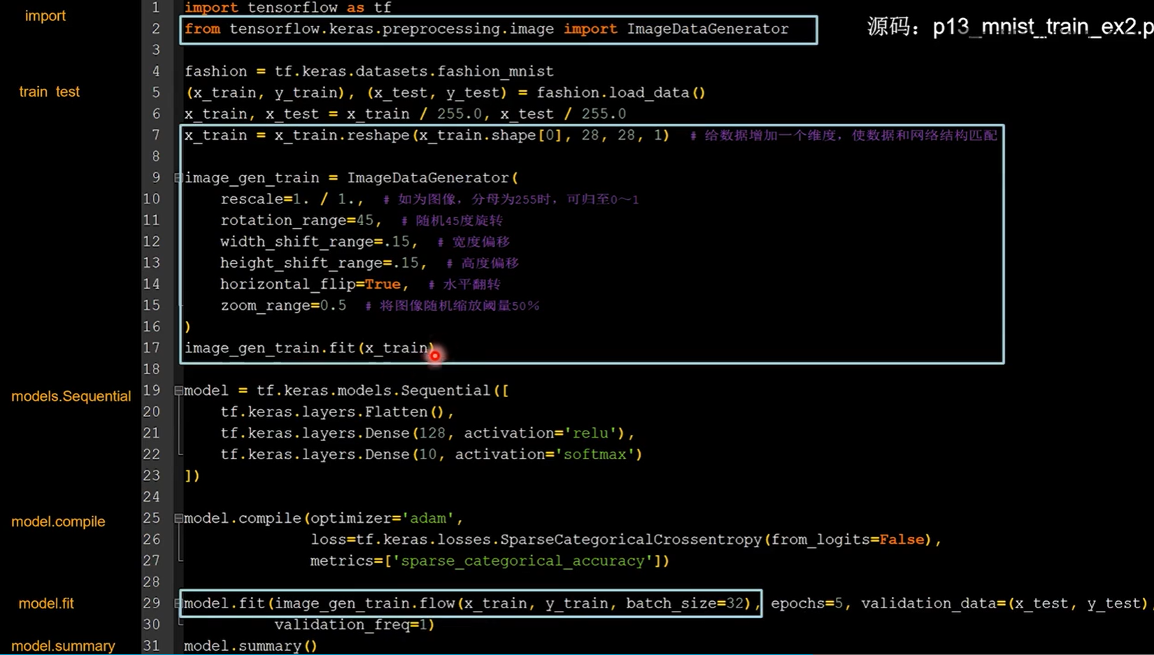
import tensorflow as tf
from tensorflow.keras.preprocessing.image import ImageDataGenerator

mnist = tf.keras.datasets.mnist
(x_train, y_train), (x_test, y_test) = mnist.load_data()
x_train, x_test = x_train / 255.0, x_test / 255.0
x_train = x_train.reshape(x_train.shape[0], 28, 28, 1)  # 给数据增加一个维度,从(60000, 28, 28)reshape为(60000, 28, 28, 1)

image_gen_train = ImageDataGenerator(
    rescale=1. / 1.,            # 如为图像,分母为255时,可归至0~1
    rotation_range=45,          # 随机45度旋转
    width_shift_range=.15,      # 宽度偏移
    height_shift_range=.15,     # 高度偏移
    horizontal_flip=False,      # 水平翻转
    zoom_range=0.5              # 将图像随机缩放阈量50%
)
image_gen_train.fit(x_train)

model = tf.keras.models.Sequential([
    tf.keras.layers.Flatten(),
    tf.keras.layers.Dense(128, activation='relu'),
    tf.keras.layers.Dense(10, activation='softmax')
])

model.compile(optimizer='adam',
              loss=tf.keras.losses.SparseCategoricalCrossentropy(from_logits=False),
              metrics=['sparse_categorical_accuracy'])

model.fit(image_gen_train.flow(x_train, y_train, batch_size=32), epochs=5, validation_data=(x_test, y_test),
          validation_freq=1)
model.summary()

因为我们的训练和测试都是在标准mnist数据集上操作的,在真实的场景中未必可以取得良好效果。这还需要验证。
断点续训
读取模型
可以使用 load_weights 函数存取文件。老师的习惯如下:
- 定义存放模型的路径和文件名,命名为 ckpt 文件。
- 生成 ckpt 文件时会同步生成 index 索引表,所以判断索引表是否存在,来判断是否存在模型参数。
- 如有索引表,则直接读取 ckpt 文件中的模型参数。
checkpoint_save_path =”./checkpoint/mnist.ckpt"
if os.path.exists (checkpoint_save_path +'.index') :
	print ( -------------load the mode1------- --- ------- ' )
	model.load_weights(checkpoint_save_path)

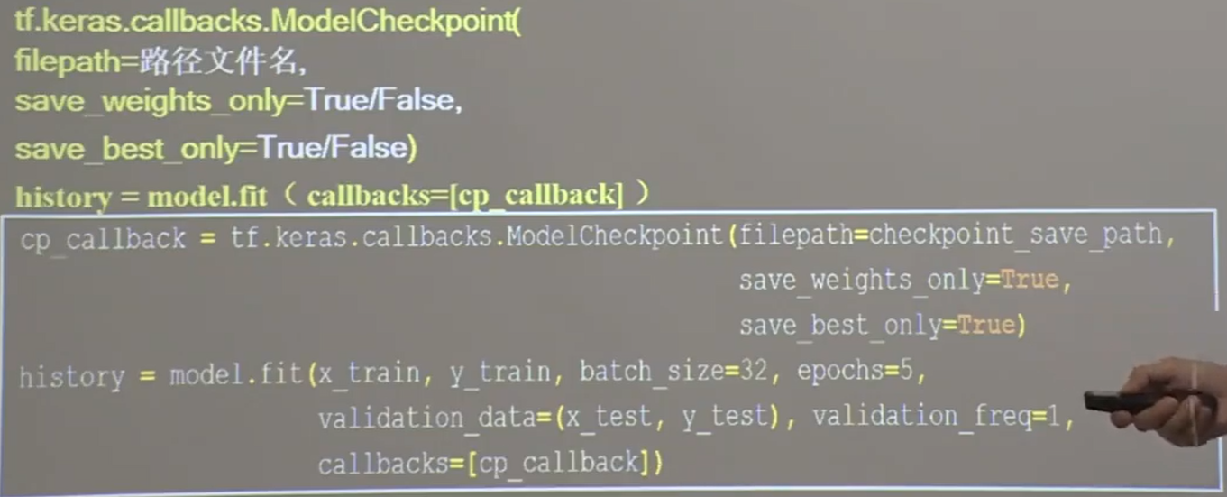
保存模型
在 callbacks.ModelCheckpoint 中可以告知一些保存参数。
可以告知文件存储路径,是否只保留模型参数,是否只保留最优结果。
cp_callback = tf.keras.callbacks.ModelCheckpoint(
	filepath=路径文件名,
	save_weights_only= True/False,  # 是否只保留模型参数
	save_best_only=True/False)  # 是否只保留最优结果

history = model.fit ( callbacks=[cp_callback] )
老师的习惯如下:
代码示例
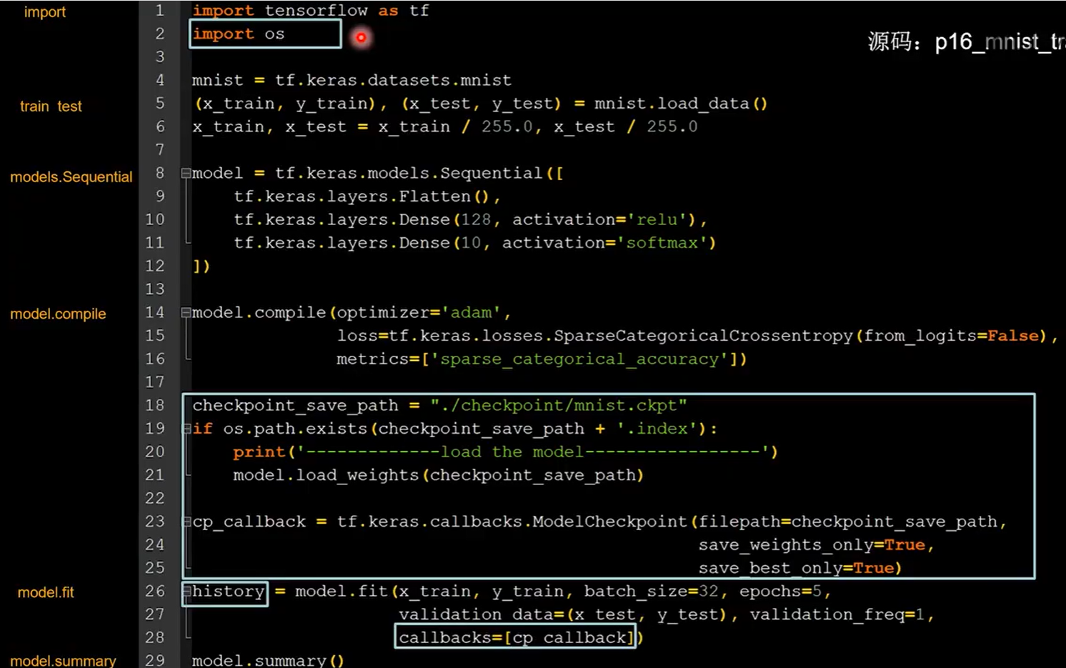
import tensorflow as tf
import os

mnist = tf.keras.datasets.mnist
(x_train, y_train), (x_test, y_test) = mnist.load_data()
x_train, x_test = x_train / 255.0, x_test / 255.0

model = tf.keras.models.Sequential([
    tf.keras.layers.Flatten(),
    tf.keras.layers.Dense(128, activation='relu'),
    tf.keras.layers.Dense(10, activation='softmax')
])

model.compile(optimizer='adam',
              loss=tf.keras.losses.SparseCategoricalCrossentropy(from_logits=False),
              metrics=['sparse_categorical_accuracy'])

checkpoint_save_path = "./checkpoint/mnist.ckpt"
if os.path.exists(checkpoint_save_path + '.index'):
    print('-------------load the model-----------------')
    model.load_weights(checkpoint_save_path)

cp_callback = tf.keras.callbacks.ModelCheckpoint(filepath=checkpoint_save_path,
                                                 save_weights_only=True,
                                                 save_best_only=True)

history = model.fit(x_train, y_train, batch_size=32, epochs=5, validation_data=(x_test, y_test), validation_freq=1,
                    callbacks=[cp_callback])
model.summary()
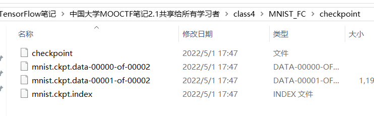
在训练过程中生成了 checkpoint 文件夹。
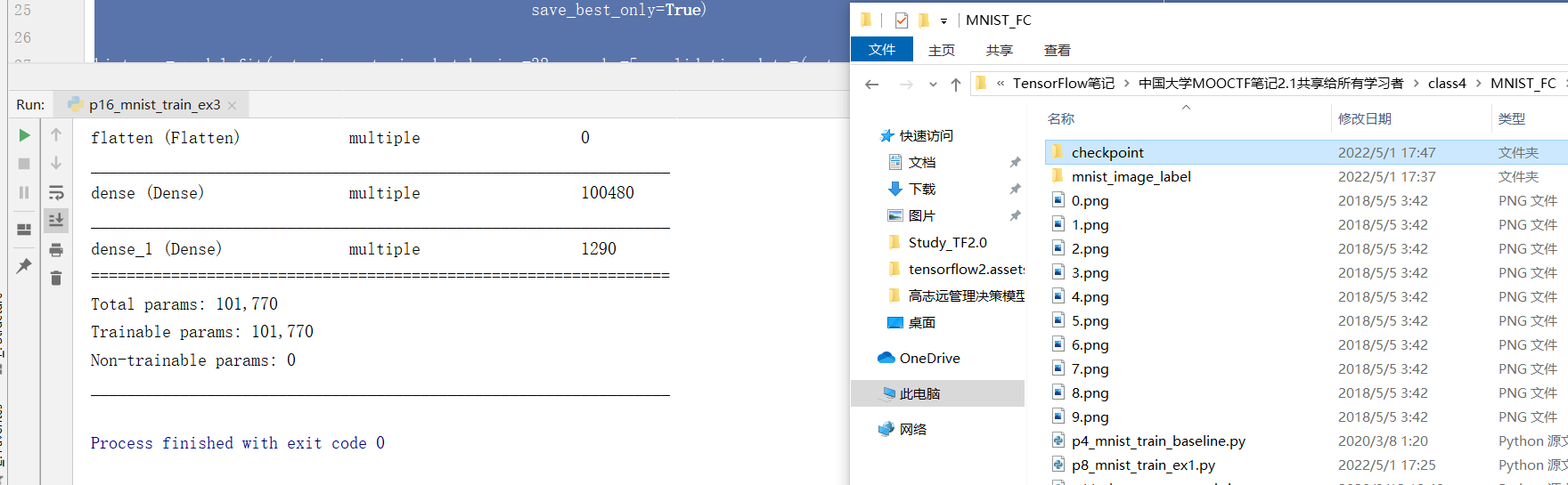
里面存放的都是模型的参数:
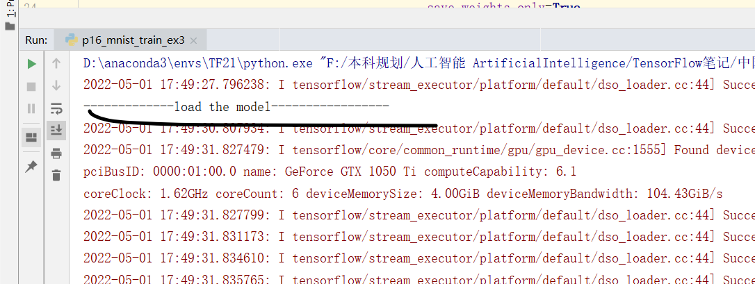
再次运行发现程序以调用刚才保存的参数:
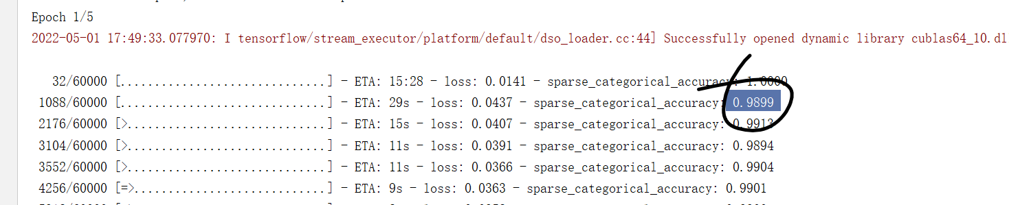
这次训练的准确率实在刚刚第一次运行的参数基础之上更近提升的:
参数提取
目的:把参数存入文本。
model.trainable_variables:返回模型中可训练的参数。
如果想看到参数可以直接print。但是有很多嘈杂内容,可以设置print输出格式:
np.set_printoptions(threshold=超过多少省略显示)
np.set_printoptions(threshold=np.inf) # np. inf表示无限大
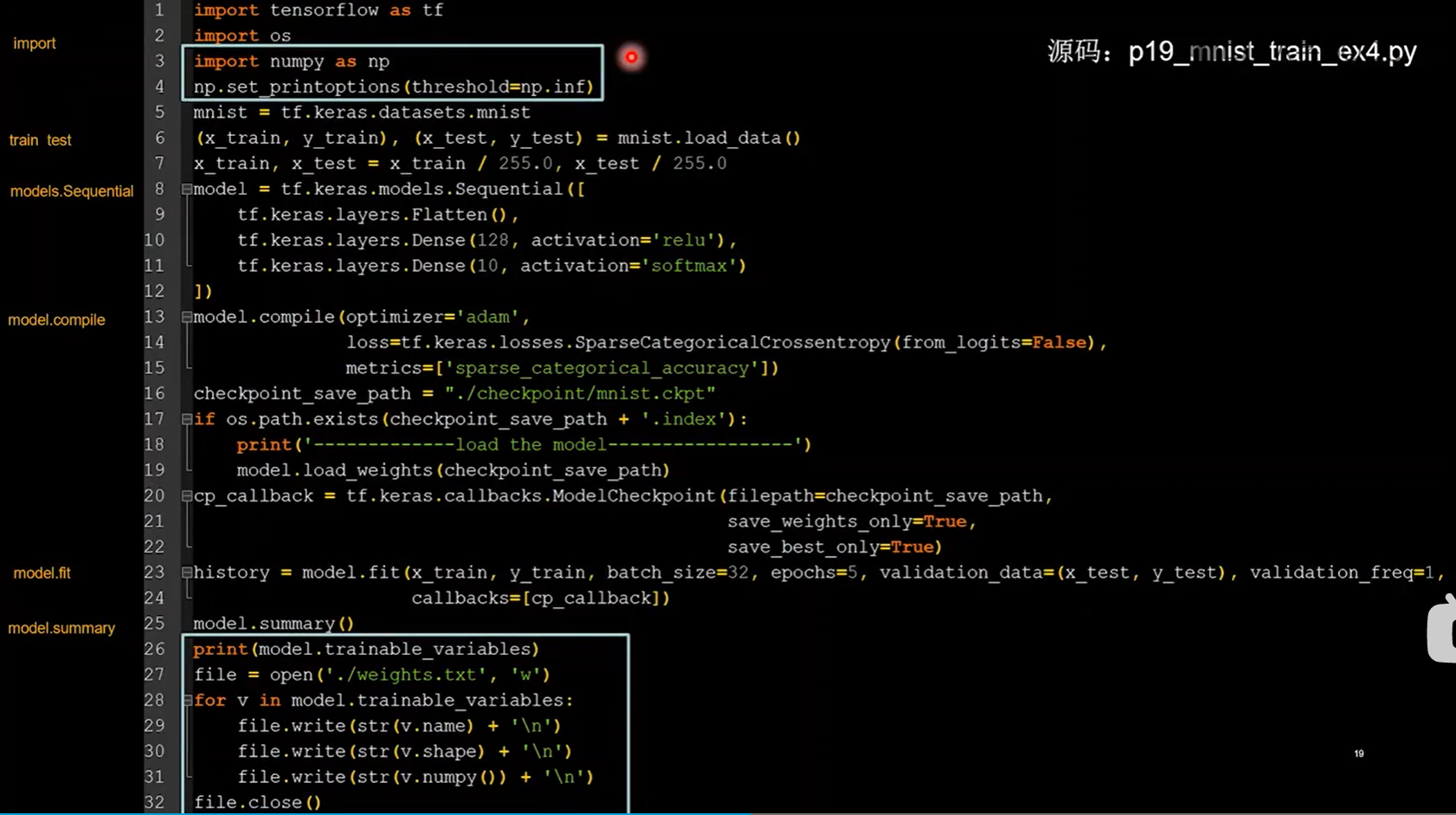
代码示例
本页代码在断点续训的基础上添加的参数提取功能。引入了numpy,print所有参数将其存入文件。
import tensorflow as tf
import os
import numpy as np
np.set_printoptions(threshold=np.inf)
mnist = tf.keras.datasets.mnist
(x_train, y_train), (x_test, y_test) = mnist.load_data()
x_train, x_test = x_train / 255.0, x_test / 255.0
model = tf.keras.models.Sequential([
    tf.keras.layers.Flatten(),
    tf.keras.layers.Dense(128, activation='relu'),
    tf.keras.layers.Dense(10, activation='softmax')
])
model.compile(optimizer='adam',
              loss=tf.keras.losses.SparseCategoricalCrossentropy(from_logits=False),
              metrics=['sparse_categorical_accuracy'])
checkpoint_save_path = "./checkpoint/mnist.ckpt"
if os.path.exists(checkpoint_save_path + '.index'):
    print('-------------load the model-----------------')
    model.load_weights(checkpoint_save_path)
cp_callback = tf.keras.callbacks.ModelCheckpoint(filepath=checkpoint_save_path,
                                                 save_weights_only=True,
                                                 save_best_only=True)
history = model.fit(x_train, y_train, batch_size=32, epochs=5, validation_data=(x_test, y_test), validation_freq=1,
                    callbacks=[cp_callback])
model.summary()

# 打印所有参数
print(model.trainable_variables)
file = open('./weights.txt', 'w')
for v in model.trainable_variables:
    file.write(str(v.name) + '\n')
    file.write(str(v.shape) + '\n')
    file.write(str(v.numpy()) + '\n')
file.close()
参数都被print打印出来并存入了txt文件:

acc/loss可视化
目标:把准确率上升和损失函数下降的过程画出来。
history=model.fit(训练集数据,训练集标签,batch_size=, epochs=,validation_split=用作测试数据的比例,validation_ data=测试集,validation_freq=测试频率)
history:
- 训练集loss: loss
- 测试集loss: val_loss
- 训练集准确率: sparse_categorical_accuracy
- 测试集准确率: val_sparse_categorical_accuracy
神经网络的八股(重要!):
import tensorflow as tf
import os
import numpy as np
from matplotlib import pyplot as plt

np.set_printoptions(threshold=np.inf)

mnist = tf.keras.datasets.mnist
(x_train, y_train), (x_test, y_test) = mnist.load_data()
x_train, x_test = x_train / 255.0, x_test / 255.0

model = tf.keras.models.Sequential([
    tf.keras.layers.Flatten(),
    tf.keras.layers.Dense(128, activation='relu'),
    tf.keras.layers.Dense(10, activation='softmax')
])

model.compile(optimizer='adam',
              loss=tf.keras.losses.SparseCategoricalCrossentropy(from_logits=False),
              metrics=['sparse_categorical_accuracy'])

checkpoint_save_path = "./checkpoint/mnist.ckpt"
if os.path.exists(checkpoint_save_path + '.index'):
    print('-------------load the model-----------------')
    model.load_weights(checkpoint_save_path)

cp_callback = tf.keras.callbacks.ModelCheckpoint(filepath=checkpoint_save_path,
                                                 save_weights_only=True,
                                                 save_best_only=True)

history = model.fit(x_train, y_train, batch_size=32, epochs=5, validation_data=(x_test, y_test), validation_freq=1,
                    callbacks=[cp_callback])
model.summary()

print(model.trainable_variables)
file = open('./weights.txt', 'w')
for v in model.trainable_variables:
    file.write(str(v.name) + '\n')
    file.write(str(v.shape) + '\n')
    file.write(str(v.numpy()) + '\n')
file.close()

###############################################    show   ###############################################

# 显示训练集和验证集的acc和loss曲线
acc = history.history['sparse_categorical_accuracy']
val_acc = history.history['val_sparse_categorical_accuracy']
loss = history.history['loss']
val_loss = history.history['val_loss']

plt.subplot(1, 2, 1)
plt.plot(acc, label='Training Accuracy')
plt.plot(val_acc, label='Validation Accuracy')
plt.title('Training and Validation Accuracy')
plt.legend()

plt.subplot(1, 2, 2)
plt.plot(loss, label='Training Loss')
plt.plot(val_loss, label='Validation Loss')
plt.title('Training and Validation Loss')
plt.legend()
plt.show()
————————以下是补充部分———————
Ps:关于plt.subplot(x, y , z),各个参数也可以用逗号,分隔开也可以写在一起。第一个参数代表子图的行数;第二个参数代表该行图像的列数; 第三个参数代表每行的第几个图像。
fig.tight_layout() # 调整整体空白
plt.subplots_adjust(wspace =0, hspace =0)  # 调整子图间距
# 参数
left  = 0.125  # the left side of the subplots of the figure
right = 0.9    # the right side of the subplots of the figure
bottom = 0.1   # the bottom of the subplots of the figure
top = 0.9      # the top of the subplots of the figure
wspace = 0.2   # the amount of width reserved for blank space between subplots,
               # expressed as a fraction of the average axis width
hspace = 0.2   # the amount of height reserved for white space between subplots,
               # expressed as a fraction of the average axis height
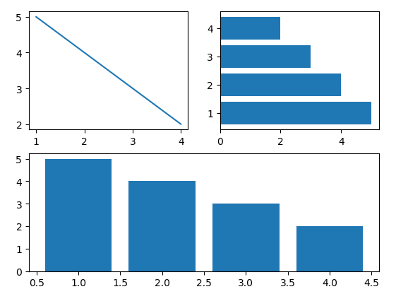
代码示例
import numpy as np
import matplotlib.pyplot as plt

x=[1,2,3,4]
y=[5,4,3,2]

plt.subplot(2,2,1) #呈现2行2列,第一行的第一幅图
plt.plot(x,y)

plt.subplot(2,2,2) #呈现2行2列,第一行的第二幅图
plt.barh(x,y)

plt.subplot(212)  # 第2行的全部
plt.bar(x,y)

plt.show()
运行结果:
acc/loss可视化代码示例
import tensorflow as tf
import os
import numpy as np
from matplotlib import pyplot as plt
np.set_printoptions(threshold=np.inf)
mnist = tf.keras.datasets.mnist
(x_train, y_train), (x_test, y_test) = mnist.load_data()
x_train, x_test = x_train / 255.0, x_test / 255.0
model = tf.keras.models.Sequential([
tf.keras.layers.Flatten(),
tf.keras.layers.Dense(128, activation='relu'),
tf.keras.layers.Dense(10, activation='softmax')
])
model.compile(optimizer='adam',
loss=tf.keras.losses.SparseCategoricalCrossentropy(from_logits=False),
metrics=['sparse_categorical_accuracy'])
checkpoint_save_path = "./checkpoint/mnist.ckpt"
if os.path.exists(checkpoint_save_path + '.index'):
print('-------------load the model-----------------')
model.load_weights(checkpoint_save_path)
cp_callback = tf.keras.callbacks.ModelCheckpoint(filepath=checkpoint_save_path,
save_weights_only=True,
save_best_only=True)
history = model.fit(x_train, y_train, batch_size=32, epochs=5, validation_data=(x_test, y_test), validation_freq=1,
callbacks=[cp_callback])
model.summary()
print(model.trainable_variables)
file = open('./weights.txt', 'w')
for v in model.trainable_variables:
file.write(str(v.name) + '\n')
file.write(str(v.shape) + '\n')
file.write(str(v.numpy()) + '\n')
file.close()
############################################### show ###############################################
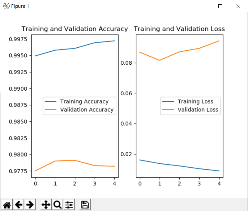
# 显示训练集和验证集的acc和loss曲线
acc = history.history['sparse_categorical_accuracy']
val_acc = history.history['val_sparse_categorical_accuracy']
loss = history.history['loss']
val_loss = history.history['val_loss']
plt.subplots_adjust( hspace =0.5)
plt.subplot(2, 1, 1)
plt.plot(acc, label='Training Accuracy')
plt.plot(val_acc, label='Validation Accuracy')
plt.title('Training and Validation Accuracy')
plt.legend()
plt.subplot(2, 1, 2)
plt.plot(loss, label='Training Loss')
plt.plot(val_loss, label='Validation Loss')
plt.title('Training and Validation Loss')
plt.legend()
plt.show()
运行结果:

编写个好用的应用程序,实现给图识物
目标:编写一个神经网络实现手写一个数字,告诉我是什么。

前向传播执行应用
predict(输入特征,batch_size=整数)
#  返回前向传播计算结果
实现步骤
# 复现模型,(前向传播)
model = tf.keras.models.Sequential([
	tf.keras.layers.Flatten(),
    tf.keras.layers.Dense(128activation='relu'),
	tf.keras.layers.Dense(10,activation='softmax')])

# 加载参数
model.load_weights(model_save_path)

# 预测结果
result = model.predict(x_ predict)
❗知识点补充:
np.newaxis:在np.newaxis所在的位置,增加一个维度
# -*- coding: utf-8 -*-
"""
tf.newaxis 和 numpy newaxis
"""
import numpy as np
import tensorflow as tf

feature = np.array([[1, 2, 3],
                        [2, 4, 6]])
center = np.array([[1, 1, 1],
                   [0, 0, 0]])

print("原始数组大小:")
print(feature.shape)
print(center.shape)

np_feature_1 = feature[:, :, np.newaxis]  # 在末尾增加一个维度
np_feature_2 = feature[:, np.newaxis] # 在中间增加一个维度
np_center = center[np.newaxis, :] # 在首部增加一个维度

print("添加 np.newaxis 后数组大小:")
print(np_feature_1.shape)
print(np_feature_1)
print('-----')
print(np_feature_2.shape)
print(np_feature_2)
print('-----')
print(np_center.shape)
print(np_center)
运行结果
原始数组大小:
(2, 3)
(2, 3)
添加 np.newaxis 后数组大小:
(2, 3, 1)
[[[1]
  [2]
  [3]]

 [[2]
  [4]
  [6]]]
-----
(2, 1, 3)
[[[1 2 3]]

 [[2 4 6]]]
-----
(1, 2, 3)
[[[1 1 1]
  [0 0 0]]]
在tensorflow中有有tf.newaxis用法相同
# -*- coding: utf-8 -*-
"""
tf.newaxis 和 numpy newaxis
"""
import numpy as np
import tensorflow as tf

feature = np.array([[1, 2, 3],
                        [2, 4, 6]])
center = np.array([[1, 1, 1],
                   [0, 0, 0]])

print("原始数组大小:")
print(feature.shape)
print(center.shape)

tf_feature_1 = feature[:, :, tf.newaxis]  # 在末尾增加一个维度
tf_feature_2 = feature[:, tf.newaxis] # 在中间增加一个维度
tf_center = center[tf.newaxis, :] # 在首部增加一个维度

print("添加 np.newaxis 后数组大小:")
print(tf_feature_1.shape)

print('-----')
print(tf_feature_2.shape)

print('-----')
print(tf_center.shape)
运行结果
原始数组大小:
(2, 3)
(2, 3)
添加 np.newaxis 后数组大小:
(2, 3, 1)
-----
(2, 1, 3)
-----
(1, 2, 3)
对于手写图片运用识别模型进行判断
from PIL import Image
import numpy as np
import tensorflow as tf
import matplotlib.pyplot as plt

model_save_path = './checkpoint/mnist.ckpt'
model = tf.keras.models.Sequential([
    tf.keras.layers.Flatten(),
    tf.keras.layers.Dense(128, activation='relu'),
    tf.keras.layers.Dense(10, activation='softmax')
])

model.load_weights(model_save_path)
preNum = int(input("input the number of test pictures:"))

for i in range(preNum):
    image_path = input("the path of test picture:")
    img = Image.open(image_path)

    image = plt.imread(image_path)
    plt.set_cmap('gray')
    plt.imshow(image)

    img = img.resize((28, 28), Image.ANTIALIAS)
    img_arr = np.array(img.convert('L'))

    # 将输入图片变为只有黑色和白色的高对比图片
    for i in range(28):
        for j in range(28):
            if img_arr[i][j] < 200:  # 小于200的变为纯黑色
                img_arr[i][j] = 255
            else:
                img_arr[i][j] = 0  # 其余变为纯白色

	# 由于神经网络训练时都是按照batch输入
    # 为了满足神经网络输入特征的shape(图片总数,宽,高)
    # 所以要将28行28列的数据[28,28]二维数据---变为--->一个28行28列的数据[1,28,28]三维数据
    img_arr = img_arr / 255.0
    x_predict = img_arr[tf.newaxis, ...]  # 插入一个维度
    result = model.predict(x_predict)
    pred = tf.argmax(result, axis=1)

    print('\n')
    tf.print(pred)

    plt.pause(1)  # 相当于plt.show(),但是只显示1秒
    plt.close()