本文已收录到:人工智能实践:Tensorflow笔记 专题
cifar10数据集
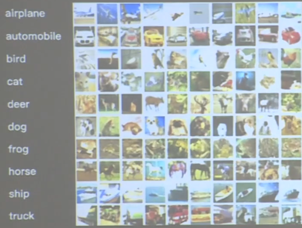
cifar10数据集一共有6万张彩色图片,每张图片有32行32列像素点的红绿蓝三通道数据。
- 提供5万张
32*32像素点的十分类彩色图片和标签,用于训练。 - 提供1万张
32*32像素点的十分类彩色图片和标签,用于测试。 - 十个分类分别是:飞机、汽车、鸟、猫、鹿、狗、青蛙、马、船和卡车,2 分别对应标签0、1、2、3一直到9
代码:
import tensorflow as tf
from matplotlib import pyplot as plt
import numpy as np
np.set_printoptions(threshold=np.inf)
# 导入cifar10数据集
cifar10 = tf.keras.datasets.cifar10
(x_train, y_train), (x_test, y_test) = cifar10.load_data()
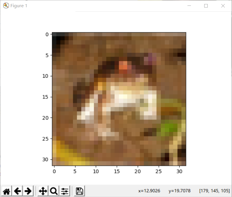
# 可视化训练集输入特征的第一个元素
plt.imshow(x_train[0]) # 绘制图片
plt.show()
# 打印出训练集输入特征的第一个元素
print("x_train[0]:\n", x_train[0])
# 打印出训练集标签的第一个元素
print("y_train[0]:\n", y_train[0])
# 打印出整个训练集输入特征形状
print("x_train.shape:\n", x_train.shape)
# 打印出整个训练集标签的形状
print("y_train.shape:\n", y_train.shape)
# 打印出整个测试集输入特征的形状
print("x_test.shape:\n", x_test.shape)
# 打印出整个测试集标签的形状
print("y_test.shape:\n", y_test.shape)
运行效果:
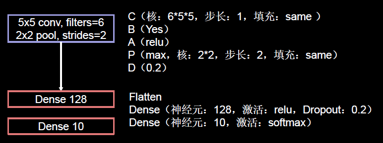
实现卷积神经网络
实现一个一层卷积、两层全连接的网络。使用6个5×5的卷积核、过2×2的池化核,池化步长是2、过128个神经元的全连接层,由于是十分类,所以最后要过10个神经元的全连接层。

用class的六步法写出代码:
"""
import
"""
import tensorflow as tf
import os
import numpy as np
from matplotlib import pyplot as plt
from tensorflow.keras.layers import Conv2D, BatchNormalization, Activation, MaxPool2D, Dropout, Flatten, Dense
from tensorflow.keras import Model
np.set_printoptions(threshold=np.inf)
"""
train test
"""
cifar10 = tf.keras.datasets.cifar10
(x_train, y_train), (x_test, y_test) = cifar10.load_data()
x_train, x_test = x_train / 255.0, x_test / 255.0
"""
class model =
"""
class Baseline(Model):
def __init__(self):
super(Baseline, self).__init__()
self.c1 = Conv2D(filters=6, kernel_size=(5, 5), padding='same') # 卷积层
self.b1 = BatchNormalization() # BN层
self.a1 = Activation('relu') # 激活层
self.p1 = MaxPool2D(pool_size=(2, 2), strides=2, padding='same') # 池化层
self.d1 = Dropout(0.2) # dropout层
self.flatten = Flatten()
self.f1 = Dense(128, activation='relu')
self.d2 = Dropout(0.2)
self.f2 = Dense(10, activation='softmax')
def call(self, x):
x = self.c1(x)
x = self.b1(x)
x = self.a1(x)
x = self.p1(x)
x = self.d1(x)
x = self.flatten(x)
x = self.f1(x)
x = self.d2(x)
y = self.f2(x)
return y
model = Baseline()
"""
model.compile 配置神经网络的训练方法
"""
model.compile(optimizer='adam',
loss=tf.keras.losses.SparseCategoricalCrossentropy(from_logits=False),
metrics=['sparse_categorical_accuracy'])
checkpoint_save_path = "./checkpoint/Baseline.ckpt"
if os.path.exists(checkpoint_save_path + '.index'):
print('-------------load the model-----------------')
model.load_weights(checkpoint_save_path)
cp_callback = tf.keras.callbacks.ModelCheckpoint(filepath=checkpoint_save_path,
save_weights_only=True,
save_best_only=True)
"""
断掉续训
"""
history = model.fit(x_train, y_train, batch_size=32, epochs=5, validation_data=(x_test, y_test), validation_freq=1,
callbacks=[cp_callback])
"""
model.summary 打印和统计
"""
model.summary()
"""
参数提取
"""
# print(model.trainable_variables)
file = open('./weights.txt', 'w')
for v in model.trainable_variables:
file.write(str(v.name) + '\n')
file.write(str(v.shape) + '\n')
file.write(str(v.numpy()) + '\n')
file.close()
"""
acc/loss可视化
"""
############################################### show ###############################################
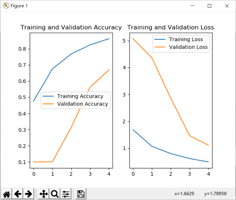
# 显示训练集和验证集的acc和loss曲线
acc = history.history['sparse_categorical_accuracy']
val_acc = history.history['val_sparse_categorical_accuracy']
loss = history.history['loss']
val_loss = history.history['val_loss']
plt.subplot(1, 2, 1)
plt.plot(acc, label='Training Accuracy')
plt.plot(val_acc, label='Validation Accuracy')
plt.title('Training and Validation Accuracy')
plt.legend()
plt.subplot(1, 2, 2)
plt.plot(loss, label='Training Loss')
plt.plot(val_loss, label='Validation Loss')
plt.title('Training and Validation Loss')
plt.legend()
plt.show()

在wedithts.tet文件里记录了所有可训练参数
- baseline/conv2d/kernel:0 (5, 5, 3, 6) 记录了第层网络用的
5*5*3的卷积核,一共6个,下边给出了这6个卷积核中的所有参数w; - baseline/conv2d/bias:0 (6,) 这里记录了6个卷积核各自的偏置项b,每个卷积核一个 b,6个卷积核共有6个偏置6 ;
- baseline/batch_normalization/gamma:0 (6,) 这里记录了BN操作中的缩放因子γ,每个卷积核一个γ,一个6个γ;
- baseline/batch_normalization/beta:0 (6,) 里记录了BN操作中的偏移因子β,每个卷积核一个β,一个6个β;
- baseline/dense/kernel:0 (1536, 128) 这里记录了第一层全链接网络,1536 行、128列的线上的权量w;
- baseline/dense/bias:0 (128,) 这里记录了第一层全连接网络128个偏置b;
- baseline/dense_1/kernel:0 (128, 10) 这里记录了第二层全链接网络,128行、10列的线上的权量w;
- baseline/dense_1/bias:0 (10,) 这里记录了第二层全连接网络10个偏置b。
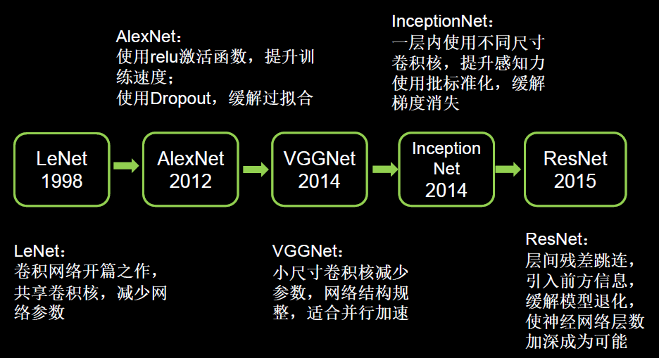
其他经典卷积网络

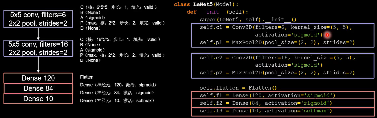
LeNet
使用两个卷积核。第一个卷积核是5×5的6个卷积核,第二层使用的事5×5的16个卷积核。Flatten构建120个神经元使用sigmoid激活,以此类推… …

代码:
import tensorflow as tf
import os
import numpy as np
from matplotlib import pyplot as plt
from tensorflow.keras.layers import Conv2D, BatchNormalization, Activation, MaxPool2D, Dropout, Flatten, Dense
from tensorflow.keras import Model

np.set_printoptions(threshold=np.inf)

cifar10 = tf.keras.datasets.cifar10
(x_train, y_train), (x_test, y_test) = cifar10.load_data()
x_train, x_test = x_train / 255.0, x_test / 255.0


class LeNet5(Model):
    def __init__(self):
        super(LeNet5, self).__init__()

        self.c1 = Conv2D(filters=6, kernel_size=(5, 5),
                         activation='sigmoid')
        self.p1 = MaxPool2D(pool_size=(2, 2), strides=2)

        self.c2 = Conv2D(filters=16, kernel_size=(5, 5),
                         activation='sigmoid')
        self.p2 = MaxPool2D(pool_size=(2, 2), strides=2)

        self.flatten = Flatten()
        self.f1 = Dense(120, activation='sigmoid')
        self.f2 = Dense(84, activation='sigmoid')
        self.f3 = Dense(10, activation='softmax')

    def call(self, x):
        x = self.c1(x)
        x = self.p1(x)

        x = self.c2(x)
        x = self.p2(x)

        x = self.flatten(x)
        x = self.f1(x)
        x = self.f2(x)
        y = self.f3(x)
        return y


model = LeNet5()

model.compile(optimizer='adam',
              loss=tf.keras.losses.SparseCategoricalCrossentropy(from_logits=False),
              metrics=['sparse_categorical_accuracy'])

checkpoint_save_path = "./checkpoint/LeNet5.ckpt"
if os.path.exists(checkpoint_save_path + '.index'):
    print('-------------load the model-----------------')
    model.load_weights(checkpoint_save_path)

cp_callback = tf.keras.callbacks.ModelCheckpoint(filepath=checkpoint_save_path,
                                                 save_weights_only=True,
                                                 save_best_only=True)

history = model.fit(x_train, y_train, batch_size=32, epochs=5, validation_data=(x_test, y_test), validation_freq=1,
                    callbacks=[cp_callback])
model.summary()

# print(model.trainable_variables)
file = open('./weights.txt', 'w')
for v in model.trainable_variables:
    file.write(str(v.name) + '\n')
    file.write(str(v.shape) + '\n')
    file.write(str(v.numpy()) + '\n')
file.close()

###############################################    show   ###############################################

# 显示训练集和验证集的acc和loss曲线
acc = history.history['sparse_categorical_accuracy']
val_acc = history.history['val_sparse_categorical_accuracy']
loss = history.history['loss']
val_loss = history.history['val_loss']

plt.subplot(1, 2, 1)
plt.plot(acc, label='Training Accuracy')
plt.plot(val_acc, label='Validation Accuracy')
plt.title('Training and Validation Accuracy')
plt.legend()

plt.subplot(1, 2, 2)
plt.plot(loss, label='Training Loss')
plt.plot(val_loss, label='Validation Loss')
plt.title('Training and Validation Loss')
plt.legend()
plt.show()
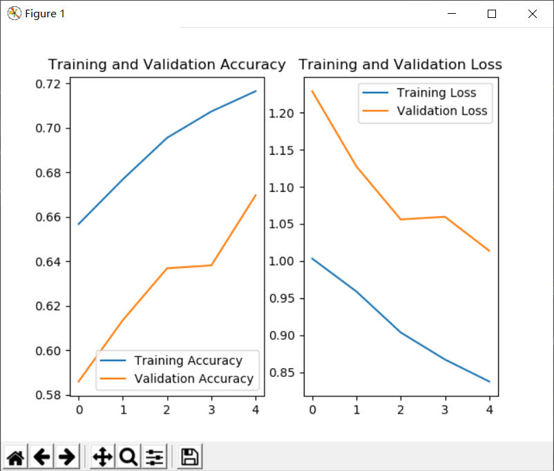
运行图:


问:正确率好低?不到50%?
答:虽然正确率还不到50%,但这是在十分类的情况下,没有做其他训练可以得到这样的结果已经很不错了。
问:为什么要设置成120、84、10这种数字?怎么来的?
答:这是从论文中复现的,适用于某种特定的数据集会达到好的效果。神经网络本来就很玄学。
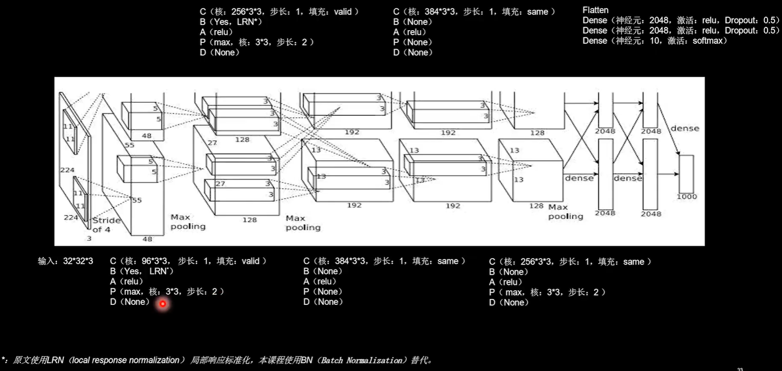
AlexNet
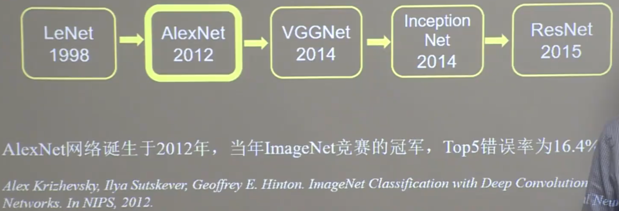
问:什么是TOP5错误率?
答:因为真实的照片中可能会有很多个标签,例如下面这张图有丁鳜鱼,但也包含了男人。
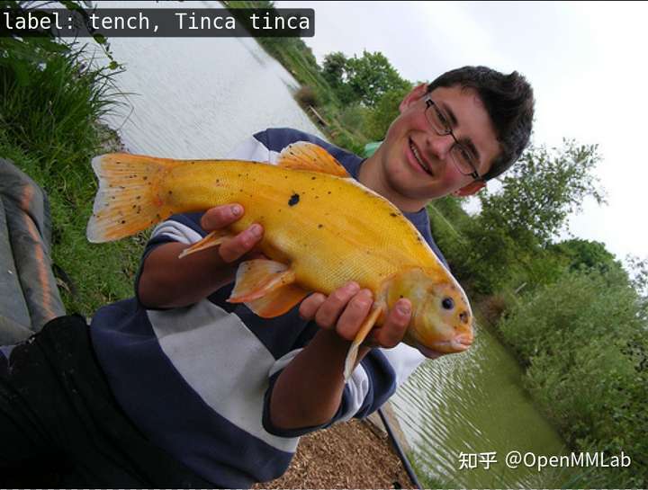
模型会预测若干个标签,TOP5错误是指正确的标签(答案)不在模型预测的前五个标签当中。

import tensorflow as tf
import os
import numpy as np
from matplotlib import pyplot as plt
from tensorflow.keras.layers import Conv2D, BatchNormalization, Activation, MaxPool2D, Dropout, Flatten, Dense
from tensorflow.keras import Model

np.set_printoptions(threshold=np.inf)

cifar10 = tf.keras.datasets.cifar10
(x_train, y_train), (x_test, y_test) = cifar10.load_data()
x_train, x_test = x_train / 255.0, x_test / 255.0


class AlexNet8(Model):
    def __init__(self):
        super(AlexNet8, self).__init__()
        self.c1 = Conv2D(filters=96, kernel_size=(3, 3))
        self.b1 = BatchNormalization()
        self.a1 = Activation('relu')
        self.p1 = MaxPool2D(pool_size=(3, 3), strides=2)

        self.c2 = Conv2D(filters=256, kernel_size=(3, 3))
        self.b2 = BatchNormalization()
        self.a2 = Activation('relu')
        self.p2 = MaxPool2D(pool_size=(3, 3), strides=2)

        self.c3 = Conv2D(filters=384, kernel_size=(3, 3), padding='same',
                         activation='relu')

        self.c4 = Conv2D(filters=384, kernel_size=(3, 3), padding='same',
                         activation='relu')

        self.c5 = Conv2D(filters=256, kernel_size=(3, 3), padding='same',
                         activation='relu')
        self.p3 = MaxPool2D(pool_size=(3, 3), strides=2)

        self.flatten = Flatten()
        self.f1 = Dense(2048, activation='relu')
        self.d1 = Dropout(0.5)
        self.f2 = Dense(2048, activation='relu')
        self.d2 = Dropout(0.5)
        self.f3 = Dense(10, activation='softmax')

    def call(self, x):
        x = self.c1(x)
        x = self.b1(x)
        x = self.a1(x)
        x = self.p1(x)

        x = self.c2(x)
        x = self.b2(x)
        x = self.a2(x)
        x = self.p2(x)

        x = self.c3(x)

        x = self.c4(x)

        x = self.c5(x)
        x = self.p3(x)

        x = self.flatten(x)
        x = self.f1(x)
        x = self.d1(x)
        x = self.f2(x)
        x = self.d2(x)
        y = self.f3(x)
        return y


model = AlexNet8()

model.compile(optimizer='adam',
              loss=tf.keras.losses.SparseCategoricalCrossentropy(from_logits=False),
              metrics=['sparse_categorical_accuracy'])

checkpoint_save_path = "./checkpoint/AlexNet8.ckpt"
if os.path.exists(checkpoint_save_path + '.index'):
    print('-------------load the model-----------------')
    model.load_weights(checkpoint_save_path)

cp_callback = tf.keras.callbacks.ModelCheckpoint(filepath=checkpoint_save_path,
                                                 save_weights_only=True,
                                                 save_best_only=True)

history = model.fit(x_train, y_train, batch_size=32, epochs=5, validation_data=(x_test, y_test), validation_freq=1,
                    callbacks=[cp_callback])
model.summary()

# print(model.trainable_variables)
file = open('./weights.txt', 'w')
for v in model.trainable_variables:
    file.write(str(v.name) + '\n')
    file.write(str(v.shape) + '\n')
    file.write(str(v.numpy()) + '\n')
file.close()

###############################################    show   ###############################################

# 显示训练集和验证集的acc和loss曲线
acc = history.history['sparse_categorical_accuracy']
val_acc = history.history['val_sparse_categorical_accuracy']
loss = history.history['loss']
val_loss = history.history['val_loss']

plt.subplot(1, 2, 1)
plt.plot(acc, label='Training Accuracy')
plt.plot(val_acc, label='Validation Accuracy')
plt.title('Training and Validation Accuracy')
plt.legend()

plt.subplot(1, 2, 2)
plt.plot(loss, label='Training Loss')
plt.plot(val_loss, label='Validation Loss')
plt.title('Training and Validation Loss')
plt.legend()
plt.show()

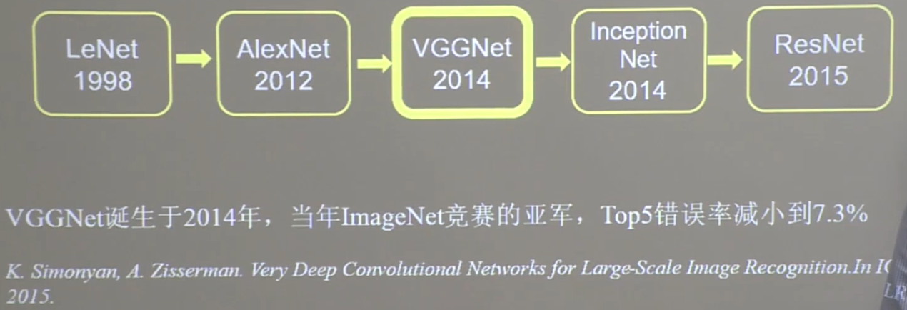
VGGNet

import tensorflow as tf
import os
import numpy as np
from matplotlib import pyplot as plt
from tensorflow.keras.layers import Conv2D, BatchNormalization, Activation, MaxPool2D, Dropout, Flatten, Dense
from tensorflow.keras import Model
np.set_printoptions(threshold=np.inf)
cifar10 = tf.keras.datasets.cifar10
(x_train, y_train), (x_test, y_test) = cifar10.load_data()
x_train, x_test = x_train / 255.0, x_test / 255.0
class VGG16(Model):
def __init__(self):
super(VGG16, self).__init__()
self.c1 = Conv2D(filters=64, kernel_size=(3, 3), padding='same') # 卷积层1
self.b1 = BatchNormalization() # BN层1
self.a1 = Activation('relu') # 激活层1
self.c2 = Conv2D(filters=64, kernel_size=(3, 3), padding='same', )
self.b2 = BatchNormalization() # BN层1
self.a2 = Activation('relu') # 激活层1
self.p1 = MaxPool2D(pool_size=(2, 2), strides=2, padding='same')
self.d1 = Dropout(0.2) # dropout层
self.c3 = Conv2D(filters=128, kernel_size=(3, 3), padding='same')
self.b3 = BatchNormalization() # BN层1
self.a3 = Activation('relu') # 激活层1
self.c4 = Conv2D(filters=128, kernel_size=(3, 3), padding='same')
self.b4 = BatchNormalization() # BN层1
self.a4 = Activation('relu') # 激活层1
self.p2 = MaxPool2D(pool_size=(2, 2), strides=2, padding='same')
self.d2 = Dropout(0.2) # dropout层
self.c5 = Conv2D(filters=256, kernel_size=(3, 3), padding='same')
self.b5 = BatchNormalization() # BN层1
self.a5 = Activation('relu') # 激活层1
self.c6 = Conv2D(filters=256, kernel_size=(3, 3), padding='same')
self.b6 = BatchNormalization() # BN层1
self.a6 = Activation('relu') # 激活层1
self.c7 = Conv2D(filters=256, kernel_size=(3, 3), padding='same')
self.b7 = BatchNormalization()
self.a7 = Activation('relu')
self.p3 = MaxPool2D(pool_size=(2, 2), strides=2, padding='same')
self.d3 = Dropout(0.2)
self.c8 = Conv2D(filters=512, kernel_size=(3, 3), padding='same')
self.b8 = BatchNormalization() # BN层1
self.a8 = Activation('relu') # 激活层1
self.c9 = Conv2D(filters=512, kernel_size=(3, 3), padding='same')
self.b9 = BatchNormalization() # BN层1
self.a9 = Activation('relu') # 激活层1
self.c10 = Conv2D(filters=512, kernel_size=(3, 3), padding='same')
self.b10 = BatchNormalization()
self.a10 = Activation('relu')
self.p4 = MaxPool2D(pool_size=(2, 2), strides=2, padding='same')
self.d4 = Dropout(0.2)
self.c11 = Conv2D(filters=512, kernel_size=(3, 3), padding='same')
self.b11 = BatchNormalization() # BN层1
self.a11 = Activation('relu') # 激活层1
self.c12 = Conv2D(filters=512, kernel_size=(3, 3), padding='same')
self.b12 = BatchNormalization() # BN层1
self.a12 = Activation('relu') # 激活层1
self.c13 = Conv2D(filters=512, kernel_size=(3, 3), padding='same')
self.b13 = BatchNormalization()
self.a13 = Activation('relu')
self.p5 = MaxPool2D(pool_size=(2, 2), strides=2, padding='same')
self.d5 = Dropout(0.2)
self.flatten = Flatten()
self.f1 = Dense(512, activation='relu')
self.d6 = Dropout(0.2)
self.f2 = Dense(512, activation='relu')
self.d7 = Dropout(0.2)
self.f3 = Dense(10, activation='softmax')
def call(self, x):
x = self.c1(x)
x = self.b1(x)
x = self.a1(x)
x = self.c2(x)
x = self.b2(x)
x = self.a2(x)
x = self.p1(x)
x = self.d1(x)
x = self.c3(x)
x = self.b3(x)
x = self.a3(x)
x = self.c4(x)
x = self.b4(x)
x = self.a4(x)
x = self.p2(x)
x = self.d2(x)
x = self.c5(x)
x = self.b5(x)
x = self.a5(x)
x = self.c6(x)
x = self.b6(x)
x = self.a6(x)
x = self.c7(x)
x = self.b7(x)
x = self.a7(x)
x = self.p3(x)
x = self.d3(x)
x = self.c8(x)
x = self.b8(x)
x = self.a8(x)
x = self.c9(x)
x = self.b9(x)
x = self.a9(x)
x = self.c10(x)
x = self.b10(x)
x = self.a10(x)
x = self.p4(x)
x = self.d4(x)
x = self.c11(x)
x = self.b11(x)
x = self.a11(x)
x = self.c12(x)
x = self.b12(x)
x = self.a12(x)
x = self.c13(x)
x = self.b13(x)
x = self.a13(x)
x = self.p5(x)
x = self.d5(x)
x = self.flatten(x)
x = self.f1(x)
x = self.d6(x)
x = self.f2(x)
x = self.d7(x)
y = self.f3(x)
return y
model = VGG16()
model.compile(optimizer='adam',
loss=tf.keras.losses.SparseCategoricalCrossentropy(from_logits=False),
metrics=['sparse_categorical_accuracy'])
checkpoint_save_path = "./checkpoint/VGG16.ckpt"
if os.path.exists(checkpoint_save_path + '.index'):
print('-------------load the model-----------------')
model.load_weights(checkpoint_save_path)
cp_callback = tf.keras.callbacks.ModelCheckpoint(filepath=checkpoint_save_path,
save_weights_only=True,
save_best_only=True)
history = model.fit(x_train, y_train, batch_size=32, epochs=5, validation_data=(x_test, y_test), validation_freq=1,
callbacks=[cp_callback])
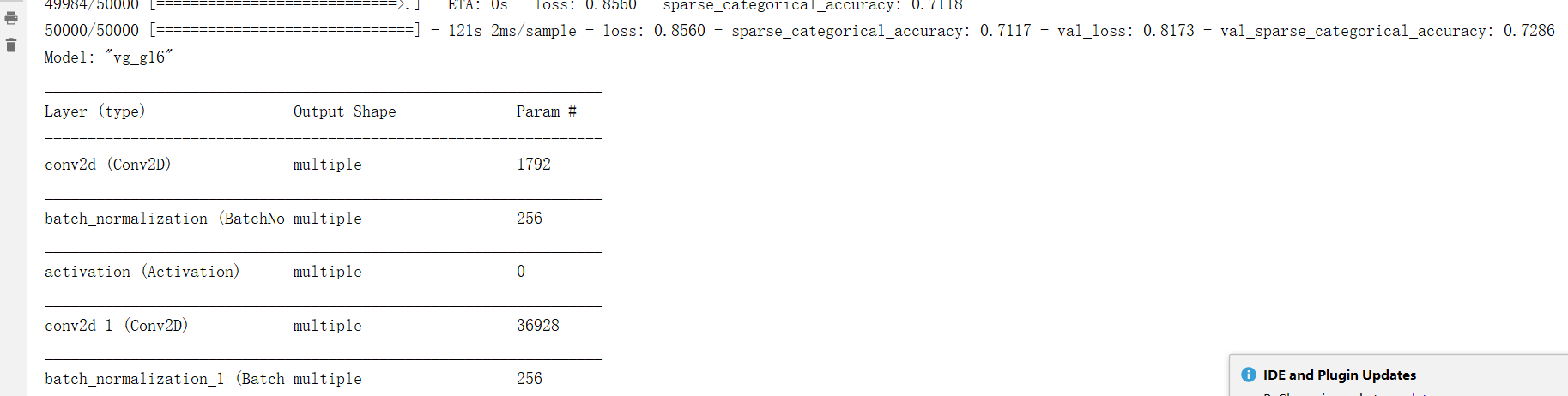
model.summary()
# print(model.trainable_variables)
file = open('./weights.txt', 'w')
for v in model.trainable_variables:
file.write(str(v.name) + '\n')
file.write(str(v.shape) + '\n')
file.write(str(v.numpy()) + '\n')
file.close()
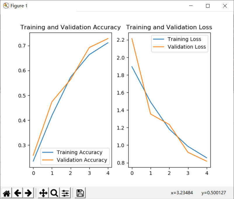
############################################### show ###############################################
# 显示训练集和验证集的acc和loss曲线
acc = history.history['sparse_categorical_accuracy']
val_acc = history.history['val_sparse_categorical_accuracy']
loss = history.history['loss']
val_loss = history.history['val_loss']
plt.subplot(1, 2, 1)
plt.plot(acc, label='Training Accuracy')
plt.plot(val_acc, label='Validation Accuracy')
plt.title('Training and Validation Accuracy')
plt.legend()
plt.subplot(1, 2, 2)
plt.plot(loss, label='Training Loss')
plt.plot(val_loss, label='Validation Loss')
plt.title('Training and Validation Loss')
plt.legend()
plt.show()
InceptionNet
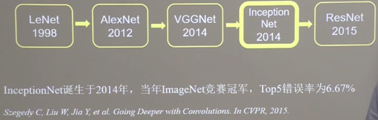
InceptionNet诞生于2014年,当年ImageNet竞赛冠军,Top5错误率为6.67%,InceptionNet 引入了 Inception结构块,在同一层网络内使用不同尺寸的卷积核,提升了模型感知力,使用了批标准化,缓解了梯度消失。
InceptionNet的核心是它的基本单元Inception结构块,无论是GoogLeNet 也就是Inception v1,还是inceptionNet的后续版本,比如v2、v3、v4,都是基于Inception结构块搭建的网络。
Inception结构块在同层网络中便用了多个尺导的卷积核,可以提取不同尺寸的特征,通过1*1卷积核,作用到输入特征图的每个像素点,通过设定少于输入特征图深度的1*1卷积核个数,减少了输出特征图深度,起到了降维的作用,减少了参数量和计算量。
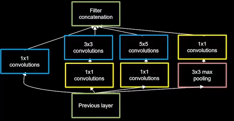
图中给出了一个Inception的结构块,Inception结构块包含四个分支,分别经过:
1*1卷积核输出到卷积连接器,1*1卷积核配合3*3卷积核输出到卷积连接器1*1卷积核配合5*5卷积核输出到卷积连接器3*3最大池化核配合1*1卷积核输出到卷积连接器
卷积连接器会把收到的这四路特征数据按深度方向拼接,形成Inception结构块的输出。

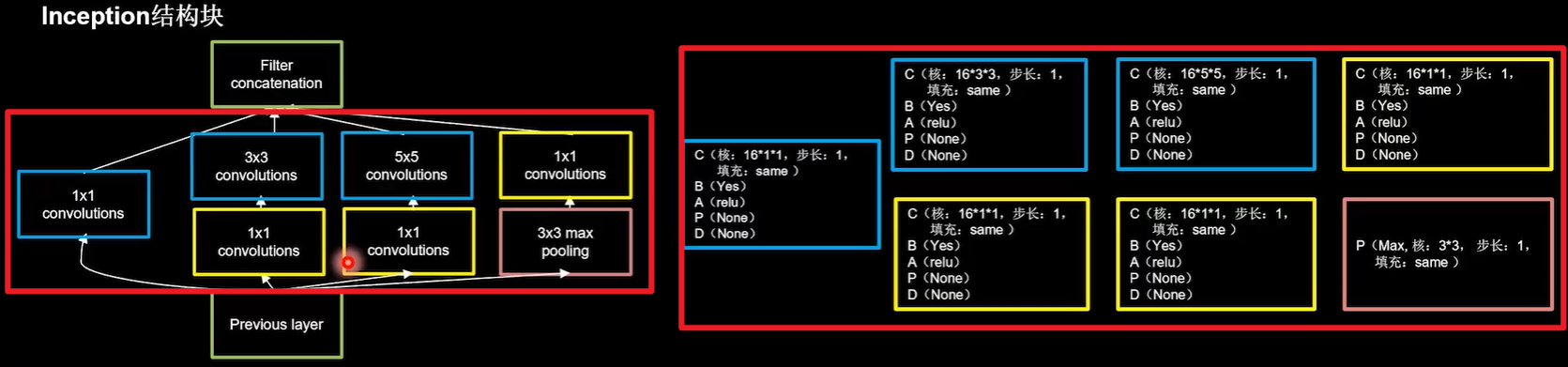
使用CBAPD将Inception结构块连接起来:
- 第一分支卷积采用了16个
1*1卷积核,步长为1全零填充,采用BN操作relu激活函数; - 第二分支先用16个
1*1卷积核降维,步长为1全零填充,采用BN操作relu激活函数;再用16个3*3卷积核,步长为1全零填充,采用BN操作relu激活函数; - 第三分支先用16个
1*1卷积核降维,步长为1全零填充,采用BN操作relu激活函数;再用16个5*5卷积核,步长为1全零填充,采用BN操作relu激活函数; - 第四分支先采用最大池化,池化核尺可是
3*3,步长为1全零填充;再用16个1*1卷积核降维,步长为1全零填充,采用BN操作relu激活函数;
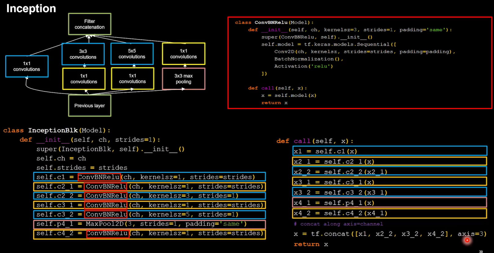
上图构思了一个Inception结构块。下面是代码的具体实现:
卷积连接器把这四个分支按照深度方向堆叠在一起,构成Inception结构块的输出,由于Inception结构块中的卷积操作均采用了CBA结构,即先卷积再BN再采用relu激活函数,所以将其定义成一个新的类ConvBNRelu,减少代码长度,增加可读性。
class ConvBNRelu(Model):
    def __init__(self, ch, kernelsz=3, strides=1, padding='same'):
        # 定义了默认卷积核边长是3步长为1全零填充
        super(ConvBNRelu, self).__init__()
        self.model = tf.keras.models.Sequential([
            Conv2D(ch, kernelsz, strides=strides, padding=padding),
            BatchNormalization(),
            Activation('relu')
        ])

    def call(self, x):
        x = self.model(x, training=False)
        #在training=False时,BN通过整个训练集计算均值、方差去做批归一化,training=True时,通过当前batch的均值、方差去做批归一化。推理时 training=False效果好
        return x
解释上面的代码:参数 ch 代表特征图的通道数,也即卷积核个数;kernelsz 代表卷积核尺寸;strides 代表卷积步长;padding 代表是否进行全零填充。 完成了这一步后,就可以开始构建 InceptionNet 的基本单元了,同样利用 class 定义的方式,定义一个新的 InceptionBlk类。
class InceptionBlk(Model):
    def __init__(self, ch, strides=1):
        super(InceptionBlk, self).__init__()
        self.ch = ch
        self.strides = strides
        self.c1 = ConvBNRelu(ch, kernelsz=1, strides=strides)
        self.c2_1 = ConvBNRelu(ch, kernelsz=1, strides=strides)
        self.c2_2 = ConvBNRelu(ch, kernelsz=3, strides=1)
        self.c3_1 = ConvBNRelu(ch, kernelsz=1, strides=strides)
        self.c3_2 = ConvBNRelu(ch, kernelsz=5, strides=1)
        self.p4_1 = MaxPool2D(3, strides=1, padding='same')
        self.c4_2 = ConvBNRelu(ch, kernelsz=1, strides=strides)

    def call(self, x):
        x1 = self.c1(x)
        x2_1 = self.c2_1(x)
        x2_2 = self.c2_2(x2_1)
        x3_1 = self.c3_1(x)
        x3_2 = self.c3_2(x3_1)
        x4_1 = self.p4_1(x)
        x4_2 = self.c4_2(x4_1)
        # concat along axis=channel
        x = tf.concat([x1, x2_2, x3_2, x4_2], axis=3)
        return x
解释上面代码:参数 ch 仍代表通道数,strides 代表卷积步长,与 ConvBNRelu 类中一致;
tf.concat 函数将四个输出按照深度方向连接在一起,x1、x2_2、x3_2、x4_2 分别代表四列输出,结合结构图和代码很容易看出二者的对应关系。
InceptionNet 网络的主体就是由其基本单元构成的,有了Inception结构块后,就可以搭建出一个精简版本的InceptionNet,网络共有10层,其模型结构如图:
解释下图:
第一层采用16个3*3卷积核,步长为1,全零填充,BN操作,rule激活。
随后是4个Inception结构块顺序相连,每两个Inception结构块组成一个block,每个bIock中的第一个Inception结构块,卷积步长是2,第二个Inception结构块,卷积步长是1,这使得第一个Inception结构块输出特征图尺寸减半,因此把输出特征图深度加深,尽可能保证特征抽取中信息的承载量一致。
block_0设置的通道数是16,经过了四个分支,输出的深度为4*16=64;在self.out_channels *= 2给通道数加倍了,所以block_1通道数是block_0通道数的两倍是32,经过了四个分支,输出的深度为4*32=128,这128个通道的数据会被送入平均池化,送入10个分类的全连接。

上面是构思,下面是代码实现:
class Inception10(Model):
    def __init__(self, num_blocks, num_classes, init_ch=16, **kwargs):
        super(Inception10, self).__init__(**kwargs)
        self.in_channels = init_ch
        self.out_channels = init_ch
        self.num_blocks = num_blocks
        self.init_ch = init_ch

        # 第一层采用16个3*3卷积核,步长为1,全零填充,BN操作,rule激活。
        # 设定了默认init_ch=16,默认输出深度是16,
        # 定义ConvBNRe lu类的时候,默认卷积核边长是3步长为1全零填充,所以直接调用
        self.c1 = ConvBNRelu(init_ch)

        # 每个bIock中的第一个Inception结构块,卷积步长是2,
        # 第二个Inception结构块,卷积步长是1,
        self.blocks = tf.keras.models.Sequential()
        for block_id in range(num_blocks):
            for layer_id in range(2):
                if layer_id == 0:
                    block = InceptionBlk(self.out_channels, strides=2)
                else:
                    block = InceptionBlk(self.out_channels, strides=1)
                self.blocks.add(block)
            # enlarger out_channels per block

            # 给通道数加倍了,所以block_1通道数是block_0通道数的两倍是32
            self.out_channels *= 2

        self.p1 = GlobalAveragePooling2D()  # 128个通道的数据会被送入平均池化
        self.f1 = Dense(num_classes, activation='softmax')  # 送入10个分类的全连接。

    def call(self, x):
        x = self.c1(x)
        x = self.blocks(x)
        x = self.p1(x)
        y = self.f1(x)
        return y

model = Inception10(num_blocks=2, num_classes=10)
解释上面代码:
- 参数
num_block代表 InceptionNet 的 Block 数,每个 Block 由两个基本单元构成; num_classes=10代表分类数,对于 cifar10 数据集来说即为 10;init_ch代表初始通道数,即 InceptionNet 基本单元的初始卷积核个数。 InceptionNet 网络不再像 VGGNet 一样有三层全连接层(全连接层的参数量占 VGGNet 总参数量的 90 %),而是采用“全局平均池化+全连接层”的方式,这减少了大量的参数。
与基础代码27类似,仅仅是class InceptionBlk(Model):和 class Inception10(Model): 这两个类和与之前的基础代码不同。可以使用pycharm右键的比较工具来阅览体会:

tips:可以修改每次喂入神经网络数据的大小参数batch_size,以充分发挥显卡性能。经过测试改为1024后,1050TI显卡跑完下面的全部代码耗时不到2分钟。一般让显卡保持70-80%的利用率最合理。

全部代码:
import tensorflow as tf
import os
import numpy as np
from matplotlib import pyplot as plt
from tensorflow.keras.layers import Conv2D, BatchNormalization, Activation, MaxPool2D, Dropout, Flatten, Dense, \
    GlobalAveragePooling2D
from tensorflow.keras import Model

np.set_printoptions(threshold=np.inf)

cifar10 = tf.keras.datasets.cifar10
(x_train, y_train), (x_test, y_test) = cifar10.load_data()
x_train, x_test = x_train / 255.0, x_test / 255.0


class ConvBNRelu(Model):
    def __init__(self, ch, kernelsz=3, strides=1, padding='same'):
        # 定义了默认卷积核边长是3步长为1全零填充
        super(ConvBNRelu, self).__init__()
        self.model = tf.keras.models.Sequential([
            Conv2D(ch, kernelsz, strides=strides, padding=padding),
            BatchNormalization(),
            Activation('relu')
        ])

    def call(self, x):
        x = self.model(x, training=False) #在training=False时,BN通过整个训练集计算均值、方差去做批归一化,training=True时,通过当前batch的均值、方差去做批归一化。推理时 training=False效果好
        return x


class InceptionBlk(Model):
    def __init__(self, ch, strides=1):
        super(InceptionBlk, self).__init__()
        self.ch = ch
        self.strides = strides
        self.c1 = ConvBNRelu(ch, kernelsz=1, strides=strides)
        self.c2_1 = ConvBNRelu(ch, kernelsz=1, strides=strides)
        self.c2_2 = ConvBNRelu(ch, kernelsz=3, strides=1)
        self.c3_1 = ConvBNRelu(ch, kernelsz=1, strides=strides)
        self.c3_2 = ConvBNRelu(ch, kernelsz=5, strides=1)
        self.p4_1 = MaxPool2D(3, strides=1, padding='same')
        self.c4_2 = ConvBNRelu(ch, kernelsz=1, strides=strides)

    def call(self, x):
        x1 = self.c1(x)
        x2_1 = self.c2_1(x)
        x2_2 = self.c2_2(x2_1)
        x3_1 = self.c3_1(x)
        x3_2 = self.c3_2(x3_1)
        x4_1 = self.p4_1(x)
        x4_2 = self.c4_2(x4_1)
        # concat along axis=channel
        x = tf.concat([x1, x2_2, x3_2, x4_2], axis=3)
        return x


class Inception10(Model):
    def __init__(self, num_blocks, num_classes, init_ch=16, **kwargs):
        super(Inception10, self).__init__(**kwargs)
        self.in_channels = init_ch
        self.out_channels = init_ch
        self.num_blocks = num_blocks
        self.init_ch = init_ch

        # 第一层采用16个3*3卷积核,步长为1,全零填充,BN操作,rule激活。
        # 设定了默认init_ch=16,默认输出深度是16,
        # 定义ConvBNRe lu类的时候,默认卷积核边长是3步长为1全零填充,所以直接调用
        self.c1 = ConvBNRelu(init_ch)

        # 每个bIock中的第一个Inception结构块,卷积步长是2,
        # 第二个Inception结构块,卷积步长是1,
        self.blocks = tf.keras.models.Sequential()
        for block_id in range(num_blocks):
            for layer_id in range(2):
                if layer_id == 0:
                    block = InceptionBlk(self.out_channels, strides=2)
                else:
                    block = InceptionBlk(self.out_channels, strides=1)
                self.blocks.add(block)
            # enlarger out_channels per block

            # 给通道数加倍了,所以block_1通道数是block_0通道数的两倍是32
            self.out_channels *= 2

        self.p1 = GlobalAveragePooling2D()  # 128个通道的数据会被送入平均池化
        self.f1 = Dense(num_classes, activation='softmax')  # 送入10个分类的全连接。

    def call(self, x):
        x = self.c1(x)
        x = self.blocks(x)
        x = self.p1(x)
        y = self.f1(x)
        return y

# num_blocks指定inceptionNet的Block数是2,block_0和block_1;
# num_classes指定网络10分类
model = Inception10(num_blocks=2, num_classes=10)

model.compile(optimizer='adam',
              loss=tf.keras.losses.SparseCategoricalCrossentropy(from_logits=False),
              metrics=['sparse_categorical_accuracy'])

checkpoint_save_path = "./checkpoint/Inception10.ckpt"
if os.path.exists(checkpoint_save_path + '.index'):
    print('-------------load the model-----------------')
    model.load_weights(checkpoint_save_path)

cp_callback = tf.keras.callbacks.ModelCheckpoint(filepath=checkpoint_save_path,
                                                 save_weights_only=True,
                                                 save_best_only=True)

history = model.fit(x_train, y_train, batch_size=1024, epochs=5, validation_data=(x_test, y_test), validation_freq=1,
                    callbacks=[cp_callback])
model.summary()

# print(model.trainable_variables)
file = open('./weights.txt', 'w')
for v in model.trainable_variables:
    file.write(str(v.name) + '\n')
    file.write(str(v.shape) + '\n')
    file.write(str(v.numpy()) + '\n')
file.close()

###############################################    show   ###############################################

# 显示训练集和验证集的acc和loss曲线
acc = history.history['sparse_categorical_accuracy']
val_acc = history.history['val_sparse_categorical_accuracy']
loss = history.history['loss']
val_loss = history.history['val_loss']

plt.subplot(1, 2, 1)
plt.plot(acc, label='Training Accuracy')
plt.plot(val_acc, label='Validation Accuracy')
plt.title('Training and Validation Accuracy')
plt.legend()

plt.subplot(1, 2, 2)
plt.plot(loss, label='Training Loss')
plt.plot(val_loss, label='Validation Loss')
plt.title('Training and Validation Loss')
plt.legend()
plt.show()

ResNet
ResNet诞生于2015年,在当年ImageNet竞赛中取得冠军,Top5错误率为3.57%。ResNet提出了层间残差跳连,引入了前方信息,缓解梯度消失,使神经网络层数增加成为可能,我们纵览刚刚讲过的四个卷积网络层数,网络层数加深提高识别准确率。
| 模型名称 | 网络层数 |
|---|---|
| LetNet | 5 |
| AlexNet | 8 |
| VGG | 16/19 |
| InceptionNet | 22 |
可见人们在探索卷积实现特征提取的道路上,通过加深网络层数,取得了越来约好的效果。
ResNet的作者何恺明在cifar10数据集上做了个实验,他发现56层卷积网络的错误率,要高于20层卷积网络的错误率,他认为单纯堆叠神经网络层数会使神经网络模型退化,以至于后边的特征丢失了前边特征的原本模样。于是他用了一根跳连线,将前边的特征直接接到了后边,使这里的输出结果H(x),包含了堆叠卷积的非线性输出F (x),和跳过这两层堆叠卷积直接连接过来的恒等映射x,让他们对应元素相加,这一操作有效缓解了神经网络模型堆叠导致的退化,使得神经网络可以向着更深层级发展。
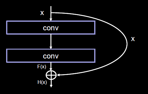
注意,ResNet块中的”+”与Inception块中的”+”是不同的
- Inception块中的“+”是沿深度方向叠加(千层蛋糕层数叠加)
- ResNet块中的“+”是特征图对应元素值相加(矩阵值相加)
ResNet块中有两种情况
一种情况用图中的实线表示,这种情况两层堆叠卷积没有改变特征图的维度,也就它们特征图的个数、高、宽和深度都相同,可以直接将F(x)与x相加。
另一种情用图中的虚线表示,这种情况中这两层堆叠卷积改变了特征图的维度,需要借助1*1的卷积来调整x的维度,使W (x)与F (x)的维度一致。
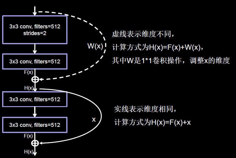
1*1卷积操作可通过步长改变特征图尺寸,通过卷积核个数改特征图深度。
ResNet块有两种形式,一种堆叠前后维度相同,另一堆叠前后维度不相同,将ResNet块的两种结构封装到一个橙色块中,定义一个ResNetBlock类,每调用一次ResNetBlock类,会生成一个黄色块。

如果堆叠卷积层前后维度不同,即residual_path等于1,调用红色块中的代码,使用1*1卷积操作,调整输入特征图inputs的尺寸或深度后,将堆叠卷积输出特征y,和if语句计算歌的residual相加、过激活、输出。
如果堆叠卷积层前后维度相同,不执行红色块内代码,直接将堆叠卷积输出特征y和输入特征图inputs相加、过激活、输出。
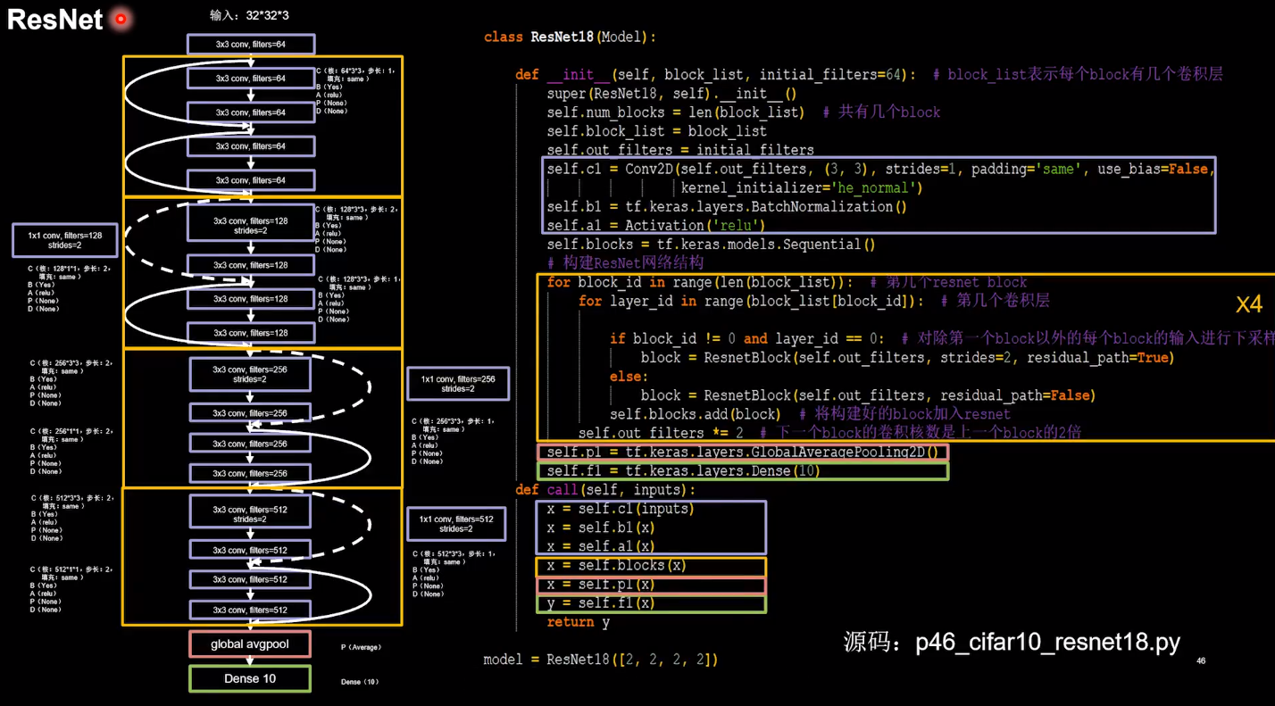
搭建网络结构。ResNet18的第一层是个卷积,然后是8个ResNet块,最后是一层全连接,每一个ResNet块有两层卷积,一共是18层网络。
第一层:采用64和3*3卷积核,步长为1,全零填充,采用BN操作,rule激活,图中代码紫色块。
下面的结果描述四个橙色块,第一个橙色快是两条实线跳连的ResNet块,第二三四个橙色快,先虚线再实线跳连的ResNet块,用for循环实现,循环次数由参赛列表元素个数决定,这里列表赋值是2,2,2,2四个元素,最外层for循环执行四次,每次进入循环,根据当前是第几个元素,选择residual_path=True,用虚线连接,residual_path=False,用实线连接,调用ReshetBlock生成左边ResNet18结构中的一个橙色块,经过平均池化和全连接,得到输出结果。
完整代码:
import tensorflow as tf
import os
import numpy as np
from matplotlib import pyplot as plt
from tensorflow.keras.layers import Conv2D, BatchNormalization, Activation, MaxPool2D, Dropout, Flatten, Dense
from tensorflow.keras import Model
np.set_printoptions(threshold=np.inf)
cifar10 = tf.keras.datasets.cifar10
(x_train, y_train), (x_test, y_test) = cifar10.load_data()
x_train, x_test = x_train / 255.0, x_test / 255.0
class ResnetBlock(Model):
def __init__(self, filters, strides=1, residual_path=False):
super(ResnetBlock, self).__init__()
self.filters = filters
self.strides = strides
self.residual_path = residual_path
self.c1 = Conv2D(filters, (3, 3), strides=strides, padding='same', use_bias=False)
self.b1 = BatchNormalization()
self.a1 = Activation('relu')
self.c2 = Conv2D(filters, (3, 3), strides=1, padding='same', use_bias=False)
self.b2 = BatchNormalization()
# residual_path为True时,对输入进行下采样,即用1x1的卷积核做卷积操作,保证x能和F(x)维度相同,顺利相加
if residual_path:
self.down_c1 = Conv2D(filters, (1, 1), strides=strides, padding='same', use_bias=False)
self.down_b1 = BatchNormalization()
self.a2 = Activation('relu')
def call(self, inputs):
residual = inputs # residual等于输入值本身,即residual=x
# 将输入通过卷积、BN层、激活层,计算F(x)
x = self.c1(inputs)
x = self.b1(x)
x = self.a1(x)
x = self.c2(x)
y = self.b2(x)
if self.residual_path:
residual = self.down_c1(inputs)
residual = self.down_b1(residual)
out = self.a2(y + residual) # 最后输出的是两部分的和,即F(x)+x或F(x)+Wx,再过激活函数
return out
class ResNet18(Model):
def __init__(self, block_list, initial_filters=64): # block_list表示每个block有几个卷积层
super(ResNet18, self).__init__()
self.num_blocks = len(block_list) # 共有几个block
self.block_list = block_list
self.out_filters = initial_filters
# 第一层
self.c1 = Conv2D(self.out_filters, (3, 3), strides=1, padding='same', use_bias=False)
self.b1 = BatchNormalization()
self.a1 = Activation('relu')
self.blocks = tf.keras.models.Sequential()
# 构建ResNet网络结构
for block_id in range(len(block_list)): # 第几个resnet block
for layer_id in range(block_list[block_id]): # 第几个卷积层
if block_id != 0 and layer_id == 0: # 对除第一个block以外的每个block的输入进行下采样
block = ResnetBlock(self.out_filters, strides=2, residual_path=True)
else:
block = ResnetBlock(self.out_filters, residual_path=False)
self.blocks.add(block) # 将构建好的block加入resnet
self.out_filters *= 2 # 下一个block的卷积核数是上一个block的2倍
self.p1 = tf.keras.layers.GlobalAveragePooling2D()
self.f1 = tf.keras.layers.Dense(10, activation='softmax', kernel_regularizer=tf.keras.regularizers.l2())
def call(self, inputs):
x = self.c1(inputs)
x = self.b1(x)
x = self.a1(x)
x = self.blocks(x)
x = self.p1(x)
y = self.f1(x)
return y
model = ResNet18([2, 2, 2, 2])
model.compile(optimizer='adam',
loss=tf.keras.losses.SparseCategoricalCrossentropy(from_logits=False),
metrics=['sparse_categorical_accuracy'])
checkpoint_save_path = "./checkpoint/ResNet18.ckpt"
if os.path.exists(checkpoint_save_path + '.index'):
print('-------------load the model-----------------')
model.load_weights(checkpoint_save_path)
cp_callback = tf.keras.callbacks.ModelCheckpoint(filepath=checkpoint_save_path,
save_weights_only=True,
save_best_only=True)
history = model.fit(x_train, y_train, batch_size=32, epochs=5, validation_data=(x_test, y_test), validation_freq=1,
callbacks=[cp_callback])
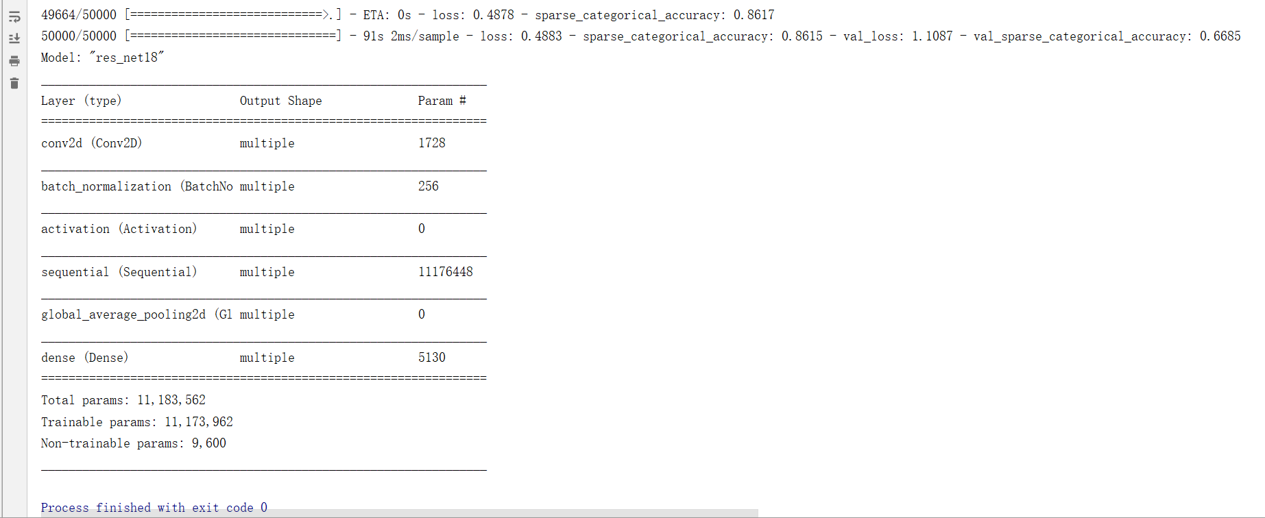
model.summary()
# print(model.trainable_variables)
file = open('./weights.txt', 'w')
for v in model.trainable_variables:
file.write(str(v.name) + '\n')
file.write(str(v.shape) + '\n')
file.write(str(v.numpy()) + '\n')
file.close()
############################################### show ###############################################
# 显示训练集和验证集的acc和loss曲线
acc = history.history['sparse_categorical_accuracy']
val_acc = history.history['val_sparse_categorical_accuracy']
loss = history.history['loss']
val_loss = history.history['val_loss']
plt.subplot(1, 2, 1)
plt.plot(acc, label='Training Accuracy')
plt.plot(val_acc, label='Validation Accuracy')
plt.title('Training and Validation Accuracy')
plt.legend()
plt.subplot(1, 2, 2)
plt.plot(loss, label='Training Loss')
plt.plot(val_loss, label='Validation Loss')
plt.title('Training and Validation Loss')
plt.legend()
plt.show()
总结
卷积是什么?卷积就是特征提取器,就是CBAPD。
卷积神经网络:借助卷积核提取空间特征后,送入全连接网络。

这种特征提取是借助卷积核实现的参数空间共享,通过卷积计算层提取空间信息。例如,我们可以用卷积核提取一张图片的空间特征,再把提取到的空间特征送入全连接网络,实现离散数据的分类。
需要注意的是,并不是每种卷积网络对所有的数据集都有很好的支持程度。这些卷积模型的提出都是当时作者针对某种特殊的数据集精挑细选参数调教出来的,并不具有通用性。例如市场上用到的模型未必都是最新的卷积模型。
参考:
https://github.com/dxc19951001/Study_TF2.0/blob/master/tensorflow2.md
https://www.bilibili.com/video/BV1B7411L7Qt?p=39